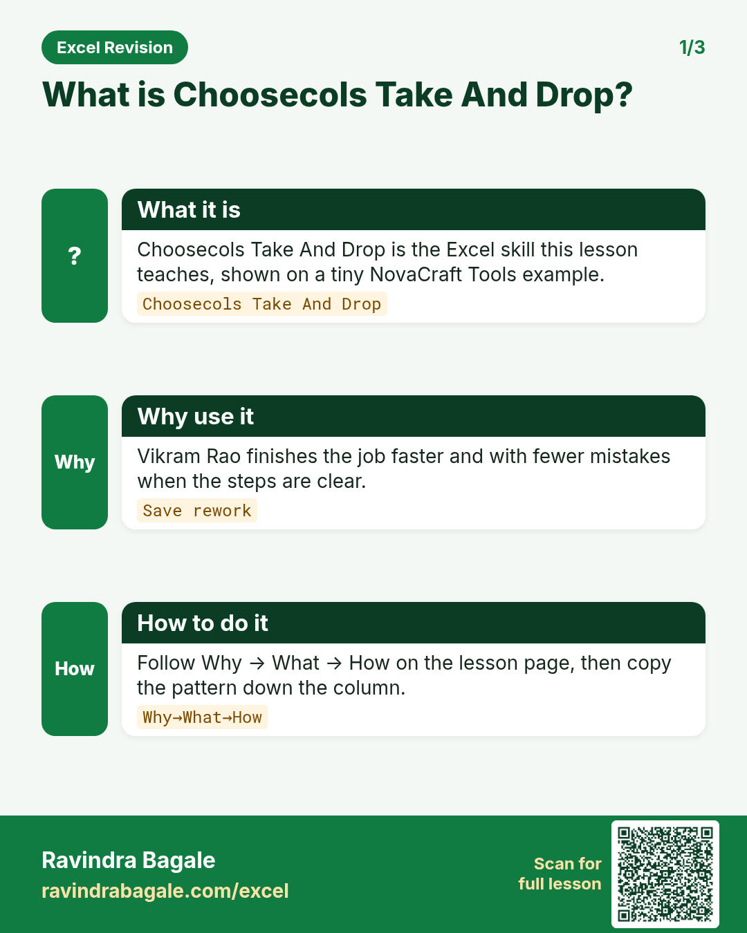
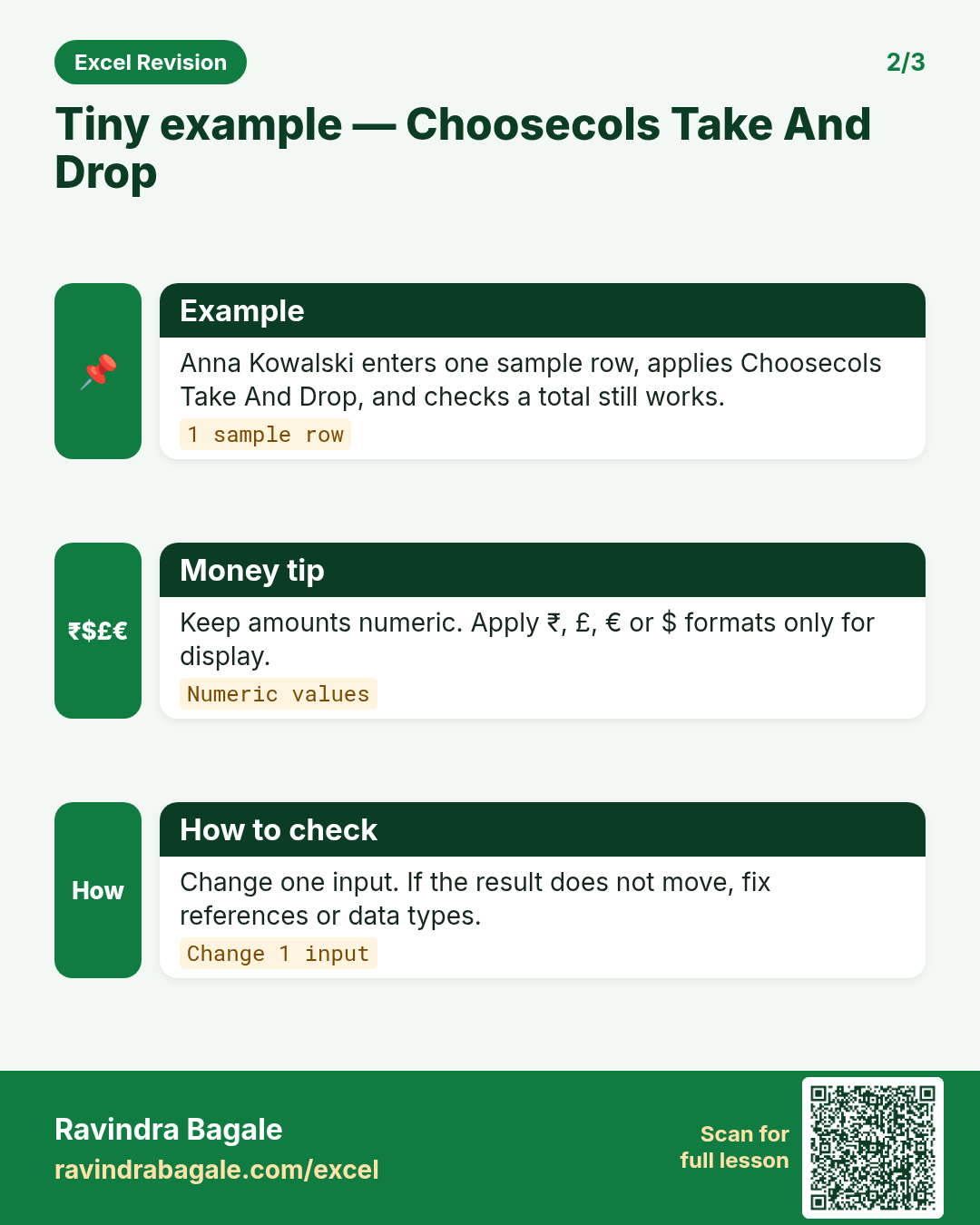
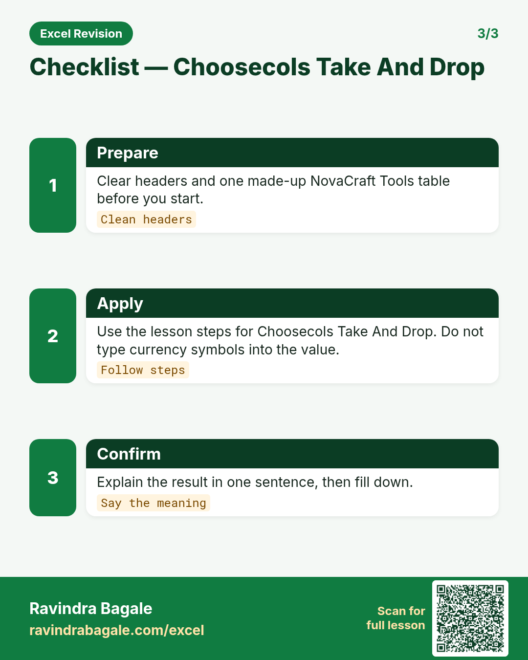
9.9 CHOOSECOLS, TAKE and DROP
Microsoft 365 / Excel 2024.
| Function | Syntax | Example | Result |
|---|---|---|---|
| CHOOSECOLS | CHOOSECOLS(array, col1, [col2], …) |
=CHOOSECOLS(tblMini, 1, 3, 7) |
Order ID, City, Amount |
| CHOOSEROWS | CHOOSEROWS(array, row1, …) |
=CHOOSEROWS(tblMini, 1, -1) |
First and last row |
| TAKE | TAKE(array, rows, [columns]) |
=TAKE(SORT(tblMini,7,-1), 3) |
Top 3 orders |
| DROP | DROP(array, rows, [columns]) |
=DROP(tblMini, 1) |
All except the first row |
About this data: Teaching sample for a fictional shop “Maple Bakery Co”. Figures and names (e.g. Rohan Patil) are made up for this lesson on choosecols take and drop.
Worked example – Top 3 orders with only three columns:
=TAKE(CHOOSECOLS(SORT(tblMini, 7, -1), 1, 3, 7), 3)
| Order ID | City | Amount |
|---|---|---|
| BLK-1007 | Solapur | 1,299 |
| BLK-1002 | Nashik | 270 |
| BLK-1004 | Nagpur | 240 |
About this data: Demo table only — not real customer or company data. Built to practise choosecols take and drop.
Negative numbers count from the end: =TAKE(tblMini, -2) returns the last two orders.
Ravindra Bagale's Tip
If you get the order of TAKE and SORT wrong, you get "the first 3 rows" instead of the "top 3" – many students apply TAKE first and then SORT. SORT first, then TAKE. Read the formula from the inside out: SORT → CHOOSECOLS → TAKE.
Ravindra Bagale's Tip – मराठी
TAKE आणि SORT ची order चुकली तर "top 3" ऐवजी "पहिल्या 3 rows" येतात – बरेच students आधी TAKE आणि मग SORT लावतात. आधी SORT, मग TAKE. Formula आतून बाहेर वाचा: SORT → CHOOSECOLS → TAKE.
Ravindra Bagale's Tip – हिंदी
TAKE और SORT का order गलत हुआ तो "top 3" की जगह "पहली 3 rows" आती हैं – बहुत से students पहले TAKE और फिर SORT लगाते हैं. पहले SORT, फिर TAKE. Formula को अंदर से बाहर पढ़ो: SORT → CHOOSECOLS → TAKE.
Practice tasks (10+)
Try these on a blank sheet. Open a hint only if you are stuck. No quiz — just practice.
1. Rebuild the smallest example of choosecols take and drop on a blank sheet for HomeNest Supplies.
Hint: Use only the steps on this page. Keep numbers numeric.
2. Change one input for Sana Sheikh and confirm the result updates.
Hint: If the result is stuck, check absolute vs relative references.
3. Repeat the same steps with a £ or € value for James O'Neill.
Hint: Formatting must not break SUM.
4. Write the result meaning in one plain sentence next to the cell.
Hint: Imagine explaining it to a new joiners.
5. Add a second row and fill the method down.
Hint: Double-click the fill handle if the pattern is consistent.
6. Break the example on purpose, then fix it using this lesson.
Hint: Common break: text instead of a number.
7. Apply choosecols take and drop to a 5-row made-up HomeNest Supplies table.
Hint: Keep column headers clear.
8. Check your answer with a simple total or COUNT.
Hint: A wrong total usually means a format or key mismatch.
9. Swap ₹ and $ on one column and re-check totals.
Hint: Stored values stay the same; only the display changes.
10. List two mistakes beginners make with choosecols take and drop.
Hint: Look back at the tip box on this page.
11. Teach the steps out loud in under one minute.
Hint: Why → What → How.
12. Save the sheet as HomeNestSup_practice.xlsx.
Hint: Use a clear file name for class.
Quick revision cards
Three standalone cards. Each one explains the idea with its own example. Scan the QR to open this lesson.