3.15 IFERROR and IFNA
IFERROR with example — in 30 seconds
What: IFERROR shows your own message when a formula returns an error.
Why: One #DIV/0! breaks the SUM below it and looks bad in a report. A clear message tells people what to fix.
Tiny example: Amount ₹90 with Qty 0 gives #DIV/0!. =IFERROR(G2/F2,"Check Qty") shows "Check Qty" instead.
IFERROR with example — 30 सेकंदात
काय: Formula ने error दिला की IFERROR तुमचा स्वतःचा message दाखवतो.
का: एक #DIV/0! खालचा SUM बिघडवतो आणि report मध्ये वाईट दिसतो. स्पष्ट message मुळे काय दुरुस्त करायचं ते कळतं.
छोटं उदाहरण: ₹90 amount आणि Qty 0 असेल तर #DIV/0! येतो. =IFERROR(G2/F2,"Check Qty") त्याऐवजी "Check Qty" दाखवतो.
IFERROR with example — 30 सेकंड में
क्या: Formula error दे तो IFERROR आपका अपना message दिखाता है.
क्यों: एक #DIV/0! नीचे का SUM बिगाड़ देता है और report में बुरा दिखता है. साफ़ message से पता चलता है कि क्या ठीक करना है.
छोटा उदाहरण: ₹90 amount और Qty 0 हो तो #DIV/0! आता है. =IFERROR(G2/F2,"Check Qty") उसकी जगह "Check Qty" दिखाता है.
First look at the data (before → after):
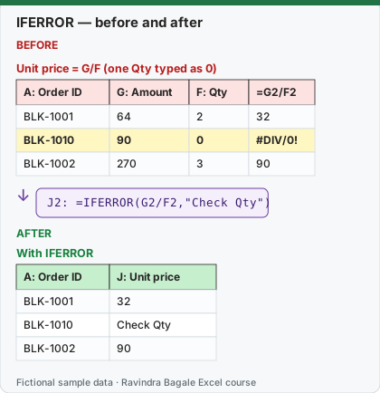
Expected result — With IFERROR
| A: Order ID | J: Unit price |
|---|---|
| BLK-1001 | 32 |
| BLK-1010 | Check Qty |
| BLK-1002 | 90 |
About this data: Teaching sample for a fictional shop “Maple Bakery Co”. Figures and names (e.g. Vikram Rao) are made up for this lesson on iferror and ifna.
Before table and formula as text
Before — Unit price = G/F (one Qty typed as 0)
| A: Order ID | G: Amount | F: Qty | =G2/F2 |
|---|---|---|---|
| BLK-1001 | 64 | 2 | 32 |
| BLK-1010 | 90 | 0 | #DIV/0! |
| BLK-1002 | 270 | 3 | 90 |
About this data: Demo table only — not real customer or company data. Built to practise iferror and ifna.
Formula / click path
J2: =IFERROR(G2/F2,"Check Qty")
Do it step by step:
- Click J2 and type
=IFERROR(G2/F2,"Check Qty"). - Press Enter and copy down.
- Filter column J for "Check Qty" to find the bad rows.
- Fix the Qty in the source data. The message disappears by itself.
- Use IFNA instead when you only want to catch #N/A from lookups.
स्टेप बाय स्टेप करून बघा:
- J2 वर click करा आणि
=IFERROR(G2/F2,"Check Qty")type करा. - Enter दाबा आणि खाली copy करा.
- Column J मध्ये "Check Qty" filter करून चुकीच्या rows शोधा.
- Source data मधली Qty दुरुस्त करा. Message आपोआप जातो.
- फक्त lookup चा #N/A पकडायचा असेल तर IFNA वापरा.
स्टेप बाय स्टेप करके देखें:
- J2 पर click करें और
=IFERROR(G2/F2,"Check Qty")type करें. - Enter दबाएँ और नीचे copy करें.
- Column J में "Check Qty" filter करके गलत rows ढूँढें.
- Source data में Qty ठीक करें. Message अपने आप चला जाता है.
- सिर्फ़ lookup का #N/A पकड़ना हो तो IFNA इस्तेमाल करें.
| Function | Catches | Example |
|---|---|---|
IFERROR(value, value_if_error) |
every error type | =IFERROR(G2/F2,0) |
IFNA(value, value_if_na) (Excel 2013+) |
only #N/A |
=IFNA(XLOOKUP(…),"Not found") |
About this data: Made-up rows so you can copy the pattern for iferror and ifna. Currencies may use ₹, £, € or $.
Worked example. Amount per unit when Qty may be blank: =IFERROR(G2/F2,"Check Qty"). Store lookup: =IFNA(VLOOKUP(A2,Stores!A:F,4,FALSE),"New store – add to master").
Ravindra Bagale's Tip
IFERROR hides every error – even a #NAME? caused by a typo or a #REF! caused by a deleted column! Many students wrap every formula in IFERROR and hide the real mistake. Use IFNA for lookups, and use IFERROR only where an error is expected.
Ravindra Bagale's Tip – मराठी
IFERROR सगळे errors लपवतो – typo मुळे आलेला #NAME? किंवा column delete केल्यामुळे आलेला #REF! सुद्धा! बरेच students सगळ्या formulas ला IFERROR लावून खरी चूक लपवतात. Lookup साठी IFNA वापरा, आणि IFERROR फक्त जिथे error अपेक्षित आहे तिथेच लावा.
Ravindra Bagale's Tip – हिंदी
IFERROR सारे errors छुपा देता है – typo से आया #NAME? या column delete होने से आया #REF! भी! बहुत से students हर formula पर IFERROR लगाकर असली गलती छुपा देते हैं. Lookup के लिए IFNA इस्तेमाल करो, और IFERROR सिर्फ़ वहीं लगाओ जहाँ error की उम्मीद हो.
Practice task
Calculate Amount/Qty with IFERROR. Look up a store's city with IFNA and show "Missing in master" for unknown store IDs.
Loading practice tasks...
- Unit price (Easy): Find the price of one item for row 2 (B2/C2).
- Shop: price per pack (Easy): Find Retail!B2/Retail!C2.
- Hide the error (Medium): For row 3, show "Check Qty" if B3/C3 gives an error.
- No error case (Medium): Use the same IFERROR formula for row 4.
- Zero instead of error (Medium): For row 3, show 0 if B3/C3 gives an error.
- Shop: no sale message (Medium): For row 3, show "No sale" if Retail!B3/Retail!C3 is an error.
- Shop: zero instead (Medium): For row 3, show 0 if Retail!B3/Retail!C3 is an error.
- Shop: normal row (Medium): Divide Retail B4 by Retail C4. If it gives an error, show "No sale".
- Not found message (Hard): Look up "BLK-1099" in A2:C4 (column 2). Show "Not found" if it is missing.
- Shop: item not stocked (Hard): Look up "Ghee" in Retail!A2:C5 (column 2). Show "Not stocked" if missing.
Quick revision cards
Three standalone cards. Each one explains the idea with its own example. Scan the QR to open this lesson.