1.8 Named Ranges
Named range with example — in 30 seconds
What: A named range gives a cell or range a friendly name, like GST_Rate, that you can use in formulas.
Why: =B2*GST_Rate is easier to read and check than =B2*Settings!$B$1. If the rate changes, you change one cell.
Tiny example: GST_Rate holds 5%. For an order of ₹270, =B2*GST_Rate gives ₹13.50.
Named range with example — 30 सेकंदात
काय: Named range म्हणजे cell किंवा range ला दिलेलं सोपं नाव, जसं GST_Rate. हे नाव formula मध्ये वापरता येतं.
का: =B2*GST_Rate वाचायला आणि check करायला =B2*Settings!$B$1 पेक्षा सोपा आहे. Rate बदलला तर फक्त एक cell बदलायची.
छोटं उदाहरण: GST_Rate मध्ये 5% आहे. ₹270 च्या order साठी =B2*GST_Rate उत्तर ₹13.50 देतो.
Named range with example — 30 सेकंड में
क्या: Named range यानी cell या range को दिया गया आसान नाम, जैसे GST_Rate. यह नाम formula में इस्तेमाल होता है.
क्यों: =B2*GST_Rate पढ़ना और check करना =B2*Settings!$B$1 से आसान है. Rate बदले तो सिर्फ़ एक cell बदलनी है.
छोटा उदाहरण: GST_Rate में 5% है. ₹270 के order के लिए =B2*GST_Rate जवाब ₹13.50 देता है.
First look at the data (before → after):
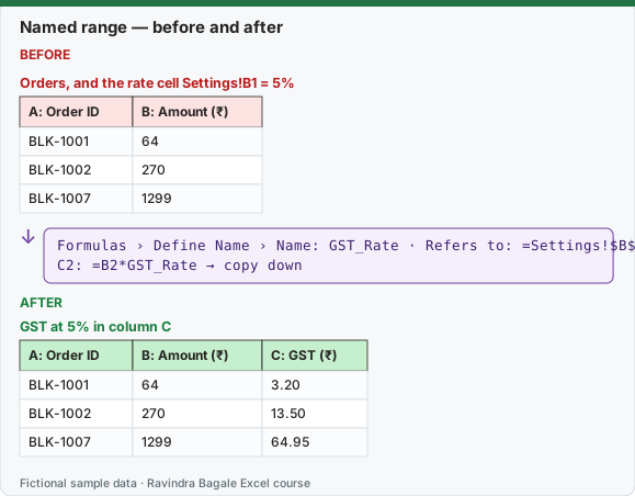
Expected result — GST at 5% in column C
| A: Order ID | B: Amount (₹) | C: GST (₹) |
|---|---|---|
| BLK-1001 | 64 | 3.20 |
| BLK-1002 | 270 | 13.50 |
| BLK-1007 | 1299 | 64.95 |
About this data: Teaching sample for a fictional shop “HomeNest Supplies”. Figures and names (e.g. Priya Deshmukh) are made up for this lesson on named ranges.
Before table and formula as text
Before — Orders, and the rate cell Settings!B1 = 5%
| A: Order ID | B: Amount (₹) |
|---|---|
| BLK-1001 | 64 |
| BLK-1002 | 270 |
| BLK-1007 | 1299 |
About this data: Demo table only — not real customer or company data. Built to practise named ranges.
Formula / click path
Formulas › Define Name › Name: GST_Rate · Refers to: =Settings!$B$1
C2: =B2*GST_Rate   → copy down
Do it step by step:
- Make a sheet named
Settingsand type5%in B1. - Click B1, then Formulas › Define Name.
- Type
GST_Ratein Name and click OK. - Go to the Orders sheet and type
=B2*GST_Ratein C2. - Copy it down. Change B1 to 12% once and watch every row update.
स्टेप बाय स्टेप करून बघा:
Settingsनावाची sheet बनवा आणि B1 मध्ये5%टाका.- B1 वर click करा, मग Formulas › Define Name.
- Name मध्ये
GST_Ratetype करा आणि OK करा. - Orders sheet वर जा आणि C2 मध्ये
=B2*GST_Ratetype करा. - तो खाली copy करा. एकदा B1 ला 12% करून बघा, सगळ्या rows बदलतात.
स्टेप बाय स्टेप करके देखें:
Settingsनाम की sheet बनाएँ और B1 में5%डालें.- B1 पर click करें, फिर Formulas › Define Name.
- Name में
GST_Ratetype करें और OK करें. - Orders sheet पर जाएँ और C2 में
=B2*GST_Ratetype करें. - इसे नीचे copy करें. एक बार B1 को 12% करके देखें, सारी rows बदल जाती हैं.
A named range gives a cell or range a meaningful name, like GST_Rate instead of $P$1.
Steps in Excel
- Quick way: select P1 › click the Name Box › type
GST_Rate› Enter. - Define Name: Formulas › Defined Names › Define Name › Name, Scope (Workbook/sheet), Refers to.
- From headers: select a table with headers › Formulas › Defined Names › Create from Selection (Ctrl + Shift + F3) › tick Top row.
- Manage/edit/delete: Formulas › Defined Names › Name Manager (Ctrl + F3).
- Use:
=K2*GST_Rate. Press F3 while typing a formula to paste a name.
Rules: names start with a letter or underscore, have no spaces (use _), and cannot look like a cell address (GST1 is fine, A1 is not).
Worked example. In Stores, Rani names B2:B16 as StoreCity and C2:C16 as StoreArea. The formula =COUNTIF(StoreCity,"Pune") returns 5 dark stores in Pune (Kothrud, Hinjewadi, Baner, Hadapsar, Wakad). Names are absolute by default, so copying the formula is safe.
Ravindra Bagale's Tip
Many students give a range a name, but when new rows are added the range doesn't grow and the new data doesn't reach the formula. For growing data, first make an Excel Table (Module 6) and use its structured reference, or update the range from Name Manager. Keep the names meaningful too – not x1 or abc.
Ravindra Bagale's Tip – मराठी
बरेच students range ला नाव देतात, पण नवीन rows add केल्यावर range वाढत नाही आणि नवीन data formula मध्ये येत नाही. वाढणाऱ्या data साठी आधी Excel Table (Module 6) बनवा आणि त्याचा structured reference वापरा, किंवा Name Manager मधून range update करा. नावंही अर्थपूर्ण ठेवा – x1, abc नको.
Ravindra Bagale's Tip – हिंदी
बहुत से students range को नाम दे देते हैं, पर नई rows जोड़ने पर range नहीं बढ़ती और नया data formula में नहीं आता. बढ़ने वाले data के लिए पहले Excel Table (Module 6) बनाओ और उसका structured reference इस्तेमाल करो, या Name Manager से range update करो. नाम भी मतलब वाले रखो – x1, abc नहीं.
Practice task
Name the GST cell GST_Rate and the Amount column OrderAmount. Write =SUM(OrderAmount)*GST_Rate. Open Name Manager and change the scope of one name to the Orders sheet only.
Thodkyaat sangaycha tar (quick recap)
Formula bar madhe khara content bagha, $ ne references lock kara (F4), ₹ aani dates format ne dakhva – type karu naka, custom format ne value na badalta display badla, Freeze Panes ne header dakhva aani named ranges ne formulas vachayla sope kara. Aata pudhe jaauya – data entry tools kade.
Loading practice tasks...
- Total parcels (Easy): Add up the "Parcels" column.
- Average cost (Easy): Average of the Cost (£) column, rounded to 2 decimals.
- Rows in Royal Mail (Easy): How many rows have Carrier "Royal Mail"?
- Largest parcels (Easy): The largest value in the "Parcels" column.
- Parcels for Royal Mail (Medium): Total of the Parcels column where Carrier is "Royal Mail".
- Royal Mail in Bristol (Medium): Total of the Parcels column where Carrier is "Royal Mail" and City is "Bristol".
- Best in Royal Mail (Medium): Largest value in the "Cost (£)" column where "Carrier" is "Royal Mail".
- Value of row 2 (Medium): Multiply the first-row Parcels by the first-row Cost (£).
- Look up Ishaan Verma (Medium): The Parcels for "Ishaan Verma" (use a lookup on the "Name" column).
- Total value (Hard): Sum of "Parcels" times "Cost (£)" for all rows.
- Share of Royal Mail (Hard): Share of the "Parcels" column that is "Royal Mail", rounded to 3 decimals.
- Share of the total "Cost (£)" with a locked range (Hard): Find what share of the total "Cost (£)" the first row has. Round it to 3 decimals.
- Above average? (Hard): "Above" if the "Cost (£)" value in the first row is above the average of the "Cost (£)" column, else "Below".
Quick revision cards
Three standalone cards. Each one explains the idea with its own example. Scan the QR to open this lesson.