1.5 Number Formats: Rupees in Indian Style and Dates
Indian rupee number format with example — in 30 seconds
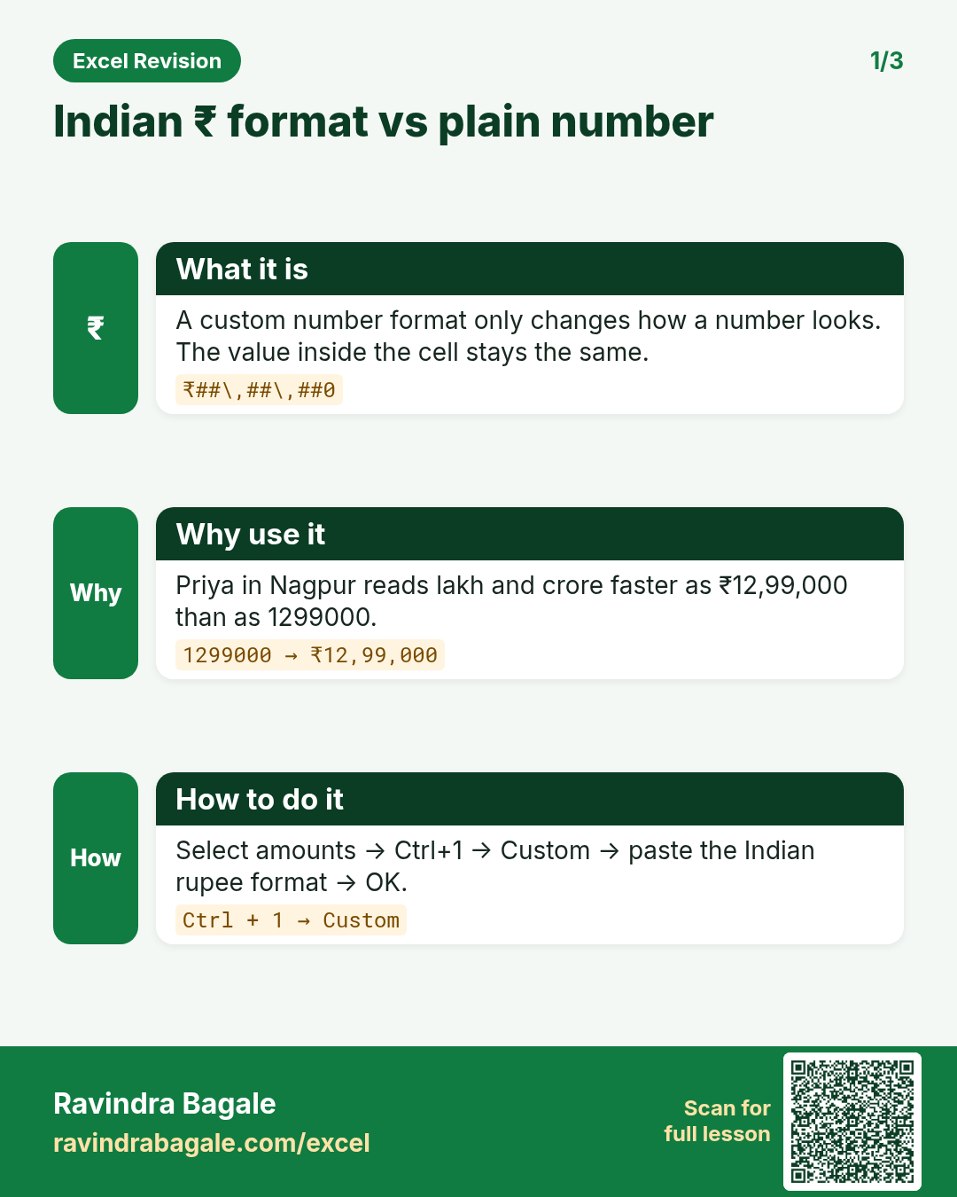
What: A custom number format changes only how a number looks. The value in the cell stays the same.
Why: Managers in Maharashtra read lakh and crore. ₹12,99,000 is easy to read; ₹1,299,000 makes people count digits.
Tiny example: The value 1299000 shows as ₹12,99,000 after you apply the custom format.
Indian rupee number format with example — 30 सेकंदात
काय: Custom number format फक्त number कसा दिसतो ते बदलतं. Cell मधली value तीच राहते.
का: महाराष्ट्रातले manager लाख आणि कोटी मध्ये वाचतात. ₹12,99,000 पटकन वाचता येतं; ₹1,299,000 बघून लोक digits मोजत बसतात.
छोटं उदाहरण: Custom format लावल्यावर 1299000 ही value ₹12,99,000 अशी दिसते.
Indian rupee number format with example — 30 सेकंड में
क्या: Custom number format सिर्फ़ number कैसा दिखता है वह बदलता है. Cell की value वही रहती है.
क्यों: महाराष्ट्र के manager लाख और करोड़ में पढ़ते हैं. ₹12,99,000 जल्दी पढ़ा जाता है; ₹1,299,000 देखकर लोग digits गिनने लगते हैं.
छोटा उदाहरण: Custom format लगाने के बाद 1299000 की value ₹12,99,000 दिखती है.
First look at the data (before → after):
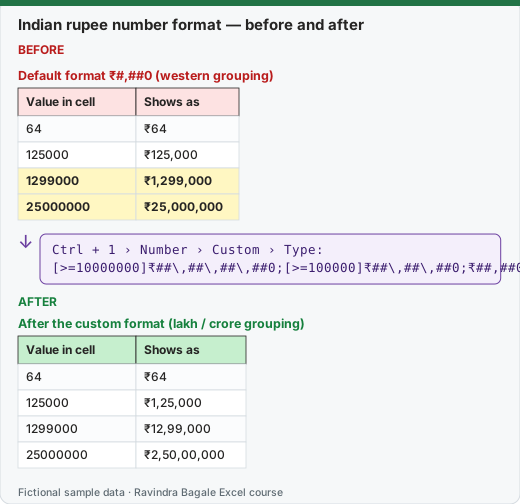
Expected result — After the custom format (lakh / crore grouping)
| Value in cell | Shows as |
|---|---|
| 64 | ₹64 |
| 125000 | ₹1,25,000 |
| 1299000 | ₹12,99,000 |
| 25000000 | ₹2,50,00,000 |
About this data: Made-up FreshGo Pune order amounts for teaching Indian comma style. Names and values are fictional.
Before table and formula as text
Before — Default format ₹#,##0 (western grouping)
| Value in cell | Shows as |
|---|---|
| 64 | ₹64 |
| 125000 | ₹125,000 |
| 1299000 | ₹1,299,000 |
| 25000000 | ₹25,000,000 |
About this data: Same fictional amounts shown with a Western thousand separator so you can compare the two looks.
Formula / click path
Ctrl + 1 › Number › Custom › Type:
[>=10000000]₹##\,##\,##\,##0;[>=100000]₹##\,##\,##0;₹##,##0
Do it step by step:
- Select the amount cells.
- Press Ctrl + 1. The Format Cells box opens.
- Click Number › Custom.
- In Type, paste the format shown in the box above.
- Click OK.
- Click one cell and look at the formula bar. The value is still a plain number, so SUM still works.
स्टेप बाय स्टेप करून बघा:
- Amount च्या cells select करा.
- Ctrl + 1 दाबा. Format Cells box उघडेल.
- Number › Custom वर click करा.
- Type मध्ये वरच्या box मधला format paste करा.
- OK वर click करा.
- एका cell वर click करून formula bar बघा. Value अजून साधा number च आहे, म्हणून SUM नीट चालतो.
स्टेप बाय स्टेप करके देखें:
- Amount वाले cells select करें.
- Ctrl + 1 दबाएँ. Format Cells box खुलेगा.
- Number › Custom पर click करें.
- Type में ऊपर वाले box का format paste करें.
- OK पर click करें.
- किसी cell पर click करके formula bar देखें. Value अभी भी सादा number है, इसलिए SUM ठीक चलता है.
Home › Number group (or Ctrl + 1 › Number tab) controls how numbers appear.
| Format | Shows 125000.5 as | Shortcut |
|---|---|---|
| General | 125000.5 | Ctrl + Shift + ~ |
| Number (2 decimals, separator) | 1,25,000.50 or 125,000.50* | Ctrl + Shift + ! |
| Currency ₹ | ₹1,25,000.50* | Ctrl + Shift + $ uses your system currency |
| Percentage | 12500050% | Ctrl + Shift + % |
| Short Date | depends on system (see below) | Ctrl + Shift + # |
About this data: Shortcut map for common number formats. The sample value 125000.5 is made up.
* Whether you see lakh grouping (1,25,000) or thousand grouping (125,000) depends on the Windows regional setting (English (India) gives 1,25,000). This may vary by version and settings.
Rupee in Indian comma style on any computer. Use this custom format (explained in 1.6):
[>=10000000]₹##\,##\,##\,##0;[>=100000]₹##\,##\,##0;₹##,##0
| Value | Displayed |
|---|---|
| 950 | ₹950 |
| 45000 | ₹45,000 |
| 125000 | ₹1,25,000 |
| 23450000 | ₹2,34,50,000 |
About this data: Worked custom-format demo using fictional ₹ sales figures from a Nashik kirana sheet.
This code handles positive numbers (the usual case for sales). If your PC is already set to English (India), the simple format ₹#,##,##0 (or ₹#,##0) also shows lakh grouping.
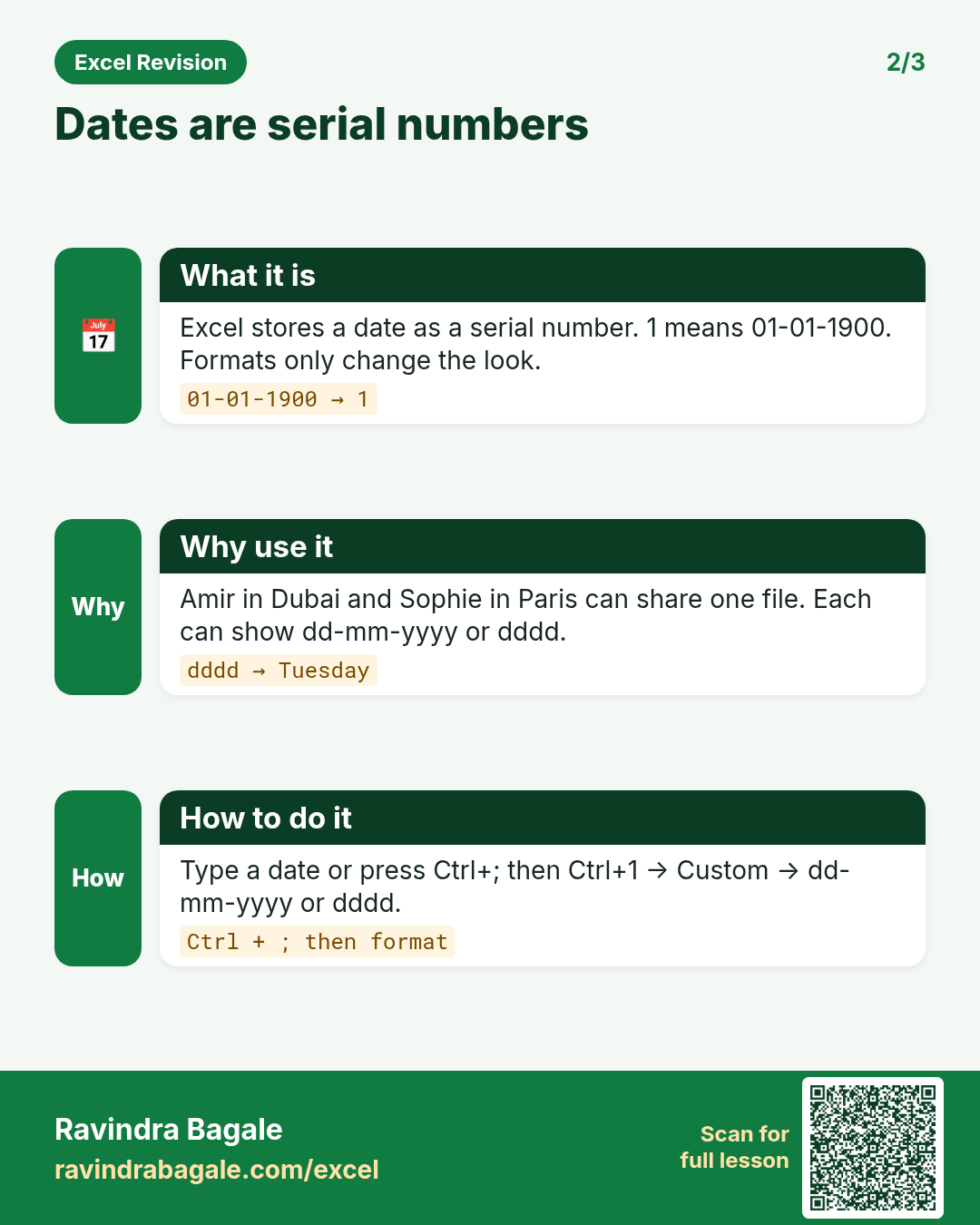
Dates. Excel stores a date as a serial number (1 = 01-01-1900) and a time as a fraction of a day (0.5 = 12:00 PM). To show dd-mm-yyyy: Ctrl + 1 › Number › Custom › type dd-mm-yyyy. For date with IST time: dd-mm-yyyy hh:mm.
Steps in Excel
- Select the Amount column › Ctrl + 1 › Number tab › Custom › paste the Indian-style code above › OK.
- Select Order Date › Ctrl + 1 › Custom ›
dd-mm-yyyy› OK. - To see the stored value, temporarily switch to General: 14-03-2026 becomes 46095.
Ravindra Bagale's Tip
Friends, many students type "₹" or "Rs." themselves in an amount – then Excel treats it as text and SUM gives 0. Type only the number in the cell, and show the ₹ symbol with a number format. In the same way, don't type a date with dots like "14.03.2026"; apply the dd-mm-yyyy format.
Ravindra Bagale's Tip – मराठी
मित्रांनो, बरेच students amount मध्ये "₹" किंवा "Rs." स्वतः type करतात – मग Excel ला तो text वाटतो आणि SUM 0 देतो. Cell मध्ये फक्त number type करा, आणि ₹ symbol number format ने दाखवा. तसंच date "14.03.2026" अशी dots ने type करू नका; dd-mm-yyyy format लावा.
Ravindra Bagale's Tip – हिंदी
दोस्तों, बहुत से students amount में "₹" या "Rs." खुद type कर देते हैं – फिर Excel उसे text मानता है और SUM 0 देता है. Cell में सिर्फ़ number type करो, और ₹ symbol number format से दिखाओ. इसी तरह date को "14.03.2026" जैसे dots से type मत करो; dd-mm-yyyy format लगाओ.
Worked example — show a London invoice in £ and a Pune bill in ₹
Why
A finance intern in Pune and a buyer in London read different money formats. The cell value must stay a pure number so SUM still works.
What
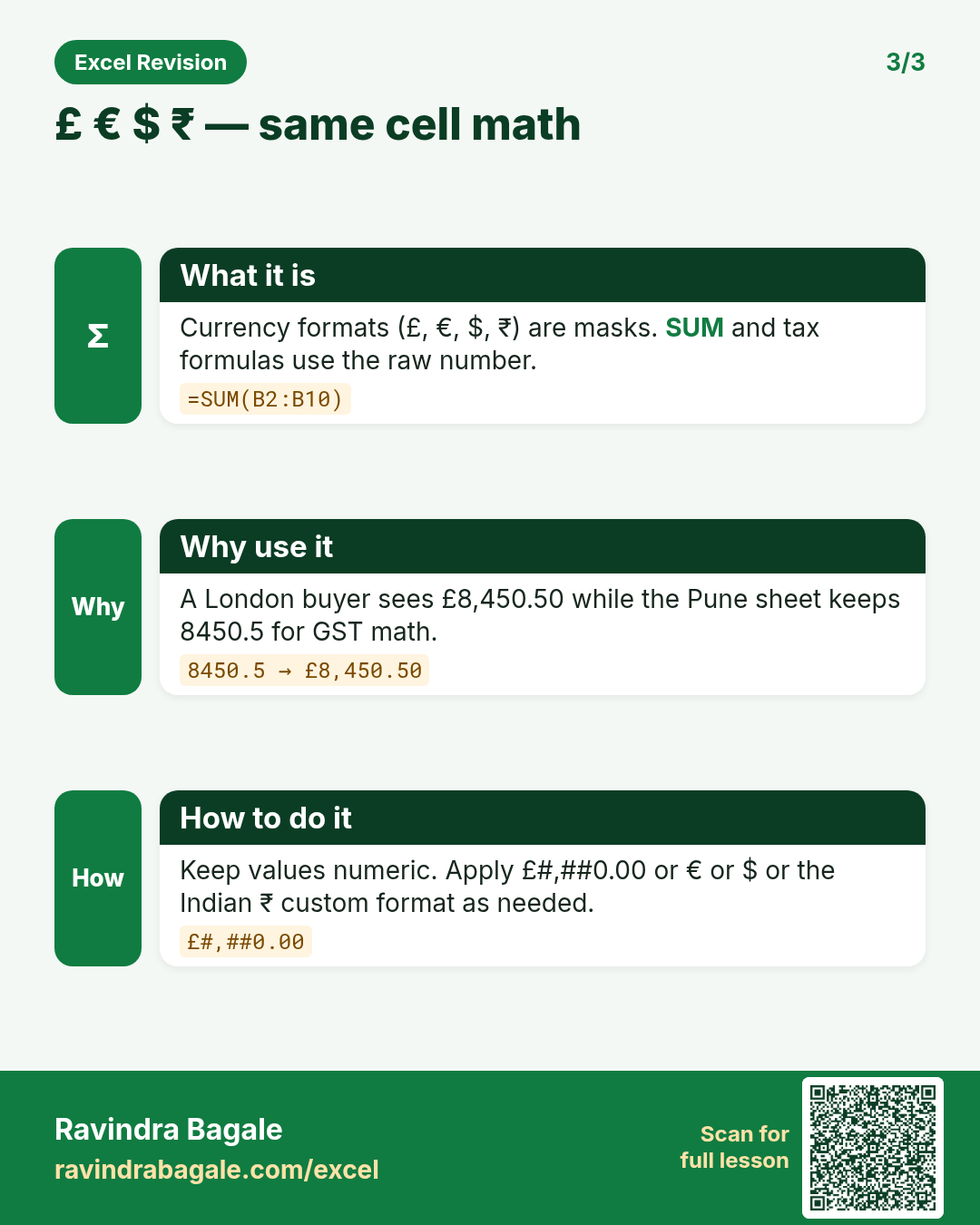
Excel number formats only change the display. We will show 1299000 as ₹12,99,000 and 8450.5 as £8,450.50.
How
- In A2 type
1299000(Priya Deshmukh's made-up QuickCart order total in ₹). - Press
Ctrl + 1→ Number → Custom. Paste the Indian rupee format from the lesson. - In B2 type
8450.5(James O'Neill's made-up UK wholesale bill). - Format B2 as
£#,##0.00(or Accounting with £). - In C2 type
=A2/100to show the value is still numeric after formatting.
Formula
=A2/100Meaning: Formatting never changes the stored number. That is why totals, tax and margins stay correct.
Practice tasks (10+)
Try these on a blank sheet. Open a hint only if you are stuck. No quiz — just practice.
1. Show 45000 as ₹45,000 with an Indian-style custom format.
Hint: Open Format Cells → Custom. Look for the lakh group pattern with ₹.
2. Show 125000 as ₹1,25,000 (not ₹125,000).
Hint: You need a format that groups by hundred after the first thousand.
3. Show 25000000 as ₹2,50,00,000.
Hint: Use the crore branch of the custom format from the lesson.
4. Type today's date with Ctrl+; and show it as dd-mm-yyyy.
Hint: After the date appears, Ctrl+1 → Custom → dd-mm-yyyy.
5. Show the same date as the day name (dddd).
Hint: Custom format dddd gives Monday, Tuesday, …
6. Format 1999.5 as £1,999.50.
Hint: Use £#,##0.00 or the Accounting format with £ symbol.
7. Format 89.9 as €89.90.
Hint: Same idea as £ — set the symbol to €.
8. In D2 put =TODAY()-Aarti's join date 15-08-2024 and show the result as a number of days.
Hint: Store the join date in a cell. Subtract from TODAY(). Format as Number.
9. Why does =SUM(A2:A5) still work after you apply ₹ formats?
Hint: Think about display vs stored value.
10. Make 0.85 show as 85% .
Hint: Ctrl+Shift+% or Format Cells → Percentage.
11. Show 1234567 as $1,234,567 (US style).
Hint: Use $#,##0 with Western grouping.
12. Enter 18:30 and show it as hh:mm AM/PM.
Hint: Excel stores time as a fraction. Use a time format.
Quick revision cards
Three standalone cards. Each one explains the idea with its own example. Scan the QR to open this lesson.