2.8 Formula-based Conditional Formatting
Formula-based conditional formatting with example — in 30 seconds
What: A formula rule colours the whole row when your formula returns TRUE for that row.
Why: Colouring only the Status cell is easy to miss. A full red row makes cancelled orders jump out.
Tiny example: In the mini sheet, Status is column I. The rule =$I2="Cancelled" paints rows BLK-1004 and BLK-1009.
Formula-based conditional formatting with example — 30 सेकंदात
काय: Formula rule मध्ये formula त्या row साठी TRUE आला की पूर्ण row रंगते.
का: फक्त Status cell रंगवली तर ती नजरेतून सुटते. पूर्ण लाल row असेल तर cancelled orders लगेच दिसतात.
छोटं उदाहरण: Mini sheet मध्ये Status column I आहे. =$I2="Cancelled" हा rule BLK-1004 आणि BLK-1009 या rows रंगवतो.
Formula-based conditional formatting with example — 30 सेकंड में
क्या: Formula rule में formula उस row के लिए TRUE आए तो पूरी row रंग जाती है.
क्यों: सिर्फ़ Status cell रंगने पर वह नज़र से छूट जाती है. पूरी लाल row से cancelled orders तुरंत दिखते हैं.
छोटा उदाहरण: Mini sheet में Status column I है. =$I2="Cancelled" rule BLK-1004 और BLK-1009 की rows रंगता है.
First look at the data (before → after):
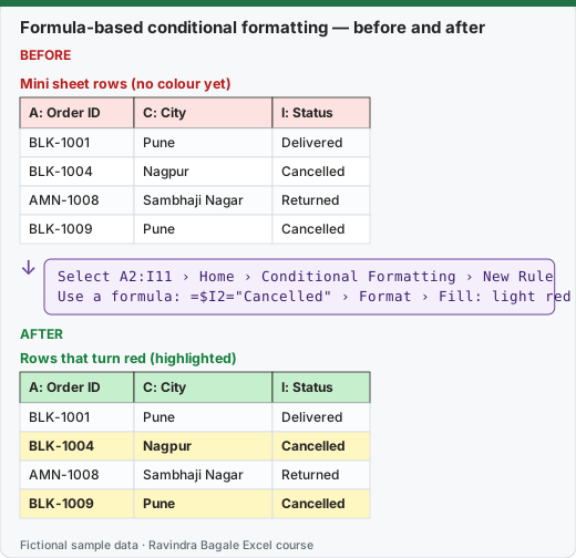
Expected result — Rows that turn red (highlighted)
| A: Order ID | C: City | I: Status |
|---|---|---|
| BLK-1001 | Pune | Delivered |
| BLK-1004 | Nagpur | Cancelled |
| AMN-1008 | Sambhaji Nagar | Returned |
| BLK-1009 | Pune | Cancelled |
About this data: Teaching sample for a fictional shop “BrightLedger Finance”. Figures and names (e.g. Rohan Patil) are made up for this lesson on formula based conditional formatting.
Before table and formula as text
Before — Mini sheet rows (no colour yet)
| A: Order ID | C: City | I: Status |
|---|---|---|
| BLK-1001 | Pune | Delivered |
| BLK-1004 | Nagpur | Cancelled |
| AMN-1008 | Sambhaji Nagar | Returned |
| BLK-1009 | Pune | Cancelled |
About this data: Demo table only — not real customer or company data. Built to practise formula based conditional formatting.
Formula / click path
Select A2:I11 › Home › Conditional Formatting › New Rule
Use a formula: =$I2="Cancelled"  › Format › Fill: light red
Do it step by step:
- Select the data A2:I11. Start from row 2, not the header.
- Click Home › Conditional Formatting › New Rule.
- Choose Use a formula to determine which cells to format.
- Type
=$I2="Cancelled". The $ locks column I; the row stays free. - Click Format › Fill, pick light red, then OK twice.
स्टेप बाय स्टेप करून बघा:
- Data A2:I11 select करा. Header नाही, row 2 पासून सुरू करा.
- Home › Conditional Formatting › New Rule वर click करा.
- Use a formula to determine which cells to format निवडा.
=$I2="Cancelled"type करा. $ मुळे column I lock होतो; row मोकळी राहते.- Format › Fill मध्ये light red निवडा, मग दोनदा OK करा.
स्टेप बाय स्टेप करके देखें:
- Data A2:I11 select करें. Header नहीं, row 2 से शुरू करें.
- Home › Conditional Formatting › New Rule पर click करें.
- Use a formula to determine which cells to format चुनें.
=$I2="Cancelled"type करें. $ से column I lock होता है; row खुली रहती है.- Format › Fill में light red चुनें, फिर दो बार OK करें.
For rules that depend on another column or a whole row, use a formula. The formula must return TRUE/FALSE and is written for the top-left cell of the selection.
Steps in Excel – highlight the entire row of cancelled orders
- Select A2:O5000 (whole data, without header).
- Home › Styles › Conditional Formatting › New Rule… › Use a formula to determine which cells to format.
- Formula:
=$N2="Cancelled"(column fixed with$, row relative). - Format… › Fill light grey, font strikethrough › OK › OK.
More formula rules on our data:
| Goal | Formula (top-left cell A2) |
|---|---|
| Late Pune deliveries | =AND($D2="Pune",$M2>15) |
| Weekend orders | =WEEKDAY($B2,2)>5 |
| Orders in Diwali week (fictional dates) | =AND($B2>=DATE(2026,11,6),$B2<=DATE(2026,11,12)) |
| Every alternate row (zebra) | =MOD(ROW(),2)=0 |
| Value above its city's average | =$K2>AVERAGEIF($D:$D,$D2,$K:$K) |
| Row matches a selected city in cell R1 | =$D2=$R$1 |
About this data: Made-up rows so you can copy the pattern for formula based conditional formatting. Currencies may use ₹, £, € or $.
Ravindra Bagale's Tip
The most common mistake in a formula rule is putting the $ in the wrong place. To colour the whole row, lock the column with $ ($N2), not the row. If you write $N$2, every row depends only on row 2 and the whole sheet turns one colour. Always write the formula for the first row of the selected range.
Ravindra Bagale's Tip – मराठी
Formula rule मध्ये सगळ्यात common चूक म्हणजे $ चुकीच्या जागी लावणं. पूर्ण row रंगवायची असेल तर column ला $ लावा ($N2), row ला नाही. $N$2 लिहिलं तर सगळ्या rows फक्त row 2 वर आधारित होतात आणि पूर्ण sheet एकाच रंगात येते. Formula नेहमी select केलेल्या range च्या पहिल्या row साठी लिहा.
Ravindra Bagale's Tip – हिंदी
Formula rule में सबसे common गलती है $ गलत जगह लगाना. पूरी row रंगनी हो तो column पर $ लगाओ ($N2), row पर नहीं. $N$2 लिखा तो सारी rows सिर्फ़ row 2 पर depend करेंगी और पूरी sheet एक ही रंग में आ जाएगी. Formula हमेशा select की गई range की पहली row के लिए लिखो.
Practice task
Highlight whole rows where Platform is MarketRush and Amount > ₹500. Then make a "selected city" cell R1 with a drop-down and highlight rows of that city only.
Loading practice tasks...
- Pass or fail (Easy): "Pass" if B2 is at least 40, else "Fail".
- Total (Easy): B2 plus C2.
- Passed score 1 (Easy): How many in B2:B11 are 40 or more?
- Passed both (Medium): TRUE if B3 and C3 are both at least 40.
- Passed either (Medium): TRUE if B4 or C4 is at least 75.
- Grade (Medium): Grade for the average of B2:C2: "A" 75+, "B" 60+, "C" 40+, else "F".
- Eligible (Medium): "Eligible" if D5 is at least 75 and B5 at least 40, else "Not eligible".
- Count passed both (Hard): How many have both scores at least 40?
- Pass percentage (Hard): Share passing score 1, rounded to 2 decimals.
- Nested IF band (Hard): "High" if C6 ≥ 75, "Mid" if ≥ 50, else "Low", using nested IF.
- Top scorer (Hard): Name with the highest score 1.
Quick revision cards
Three standalone cards. Each one explains the idea with its own example. Scan the QR to open this lesson.