5.6 Numbers Stored as Text
Numbers stored as text with example — in 30 seconds
What: A number stored as text looks like a number but Excel treats it as words. SUM skips it.
Why: Your total shows ₹0 or a too-small number, and nobody notices until the meeting.
Tiny example: Three amounts 64, 270 and 110 are text. =SUM(C2:C4) gives 0. After conversion it gives 444.
Numbers stored as text with example — 30 सेकंदात
काय: Text म्हणून साठवलेला number दिसतो number सारखा, पण Excel त्याला शब्द समजतो. SUM त्याला सोडून देतो.
का: तुमचा total ₹0 किंवा खूप कमी येतो, आणि meeting पर्यंत कुणाच्या लक्षात येत नाही.
छोटं उदाहरण: 64, 270 आणि 110 हे तीन amounts text आहेत. =SUM(C2:C4) उत्तर 0 देतो. Convert केल्यावर उत्तर 444.
Numbers stored as text with example — 30 सेकंड में
क्या: Text के रूप में रखा number दिखता number जैसा है, पर Excel उसे शब्द मानता है. SUM उसे छोड़ देता है.
क्यों: आपका total ₹0 या बहुत कम आता है, और meeting तक किसी का ध्यान नहीं जाता.
छोटा उदाहरण: 64, 270 और 110 ये तीन amounts text हैं. =SUM(C2:C4) जवाब 0 देता है. Convert करने पर जवाब 444.
First look at the data (before → after):
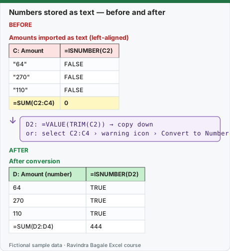
Expected result — After conversion
| D: Amount (number) | =ISNUMBER(D2) |
|---|---|
| 64 | TRUE |
| 270 | TRUE |
| 110 | TRUE |
| =SUM(D2:D4) | 444 |
About this data: Teaching sample for a fictional shop “BrightLedger Finance”. Figures and names (e.g. Sana Sheikh) are made up for this lesson on numbers stored as text.
Before table and formula as text
Before — Amounts imported as text (left-aligned)
| C: Amount | =ISNUMBER(C2) |
|---|---|
| "64" | FALSE |
| "270" | FALSE |
| "110" | FALSE |
| =SUM(C2:C4) | 0 |
About this data: Demo table only — not real customer or company data. Built to practise numbers stored as text.
Formula / click path
D2: =VALUE(TRIM(C2))   → copy down
or: select C2:C4 › warning icon › Convert to Number
Do it step by step:
- Type
=ISNUMBER(C2)next to the data. FALSE means text. - Quick fix: select the cells, click the yellow warning icon, choose Convert to Number.
- Formula fix: type
=VALUE(TRIM(C2))in D2 and copy down. - Copy column D and Paste Special › Values over column C.
- Check: the SUM now shows 444.
स्टेप बाय स्टेप करून बघा:
- Data च्या बाजूला
=ISNUMBER(C2)type करा. FALSE म्हणजे text. - पटकन fix: cells select करा, पिवळ्या warning icon वर click करा, Convert to Number निवडा.
- Formula ने fix: D2 मध्ये
=VALUE(TRIM(C2))type करा आणि खाली copy करा. - Column D copy करा आणि column C वर Paste Special › Values करा.
- Check करा: SUM आता 444 दाखवतो.
स्टेप बाय स्टेप करके देखें:
- Data के बगल में
=ISNUMBER(C2)type करें. FALSE यानी text. - जल्दी fix: cells select करें, पीले warning icon पर click करें, Convert to Number चुनें.
- Formula से fix: D2 में
=VALUE(TRIM(C2))type करें और नीचे copy करें. - Column D copy करें और column C पर Paste Special › Values करें.
- Check करें: SUM अब 444 दिखाता है.
Signs: numbers are left-aligned, a green triangle appears, SUM returns 0 or a smaller total, =ISNUMBER(C2) is FALSE.
Before
| Order ID | Amount (text) |
|---|---|
| BLK-3201 | ₹1,299 |
| BLK-3202 | Rs. 450 |
| BLK-3203 | 1,25,000 |
| BLK-3204 | '64 |
| BLK-3205 | 90 INR |
About this data: Made-up rows so you can copy the pattern for numbers stored as text. Currencies may use ₹, £, € or $.
=SUM() → 0
After
| Order ID | Amount |
|---|---|
| BLK-3201 | 1299 |
| BLK-3202 | 450 |
| BLK-3203 | 125000 |
| BLK-3204 | 64 |
| BLK-3205 | 90 |
About this data: Fictional worksheet used in class. Safe to edit; nothing here is live production data.
=SUM() → 1,26,903
Steps in Excel – four ways
- Error button: select the cells with green triangles › click ⚠ › Convert to Number (works for plain numbers like '64).
-
Formula: remove symbols, then VALUE:
=VALUE(TRIM(SUBSTITUTE(SUBSTITUTE(SUBSTITUTE(SUBSTITUTE(B2,"₹",""),"Rs.",""), "INR",""), ",",""))) -
Text to Columns: select the column › Data › Data Tools › Text to Columns › Delimited › Next › untick all delimiters › Next › General › Finish. Excel re-reads each cell as a number.
- Paste Special Multiply: type
1in an empty cell › copy it › select the text numbers › Home › Paste › Paste Special… › Multiply › OK. - Apply the rupee number format (1.5). Verify with
=SUMPRODUCT(--ISNUMBER(C2:C6))= 5.
Ravindra Bagale's Tip
Many students look at the total of the amount column and say "it's correct", but if half the cells are text, SUM skips them – the total comes out lower and nobody notices. Compare =COUNT() and =COUNTA(): if they differ, you have text-numbers. Clean numbers typed with ₹ and commas first, then apply the format.
Ravindra Bagale's Tip – मराठी
बरेच students amount column चा total बघून "बरोबर आहे" म्हणतात, पण अर्ध्या cells text असतील तर SUM त्यांना सोडून देतो – total कमी येतो आणि कोणालाच कळत नाही. =COUNT() आणि =COUNTA() compare करा: फरक असेल तर text-numbers आहेत. ₹ आणि comma type केलेले numbers आधी साफ करा, मग format लावा.
Ravindra Bagale's Tip – हिंदी
बहुत से students amount column का total देखकर "सही है" कह देते हैं, पर अगर आधी cells text हैं तो SUM उन्हें छोड़ देता है – total कम आता है और किसी को पता नहीं चलता. =COUNT() और =COUNTA() compare करो: फ़र्क हो तो text-numbers हैं. ₹ और comma के साथ type किए numbers पहले साफ़ करो, फिर format लगाओ.
Practice task
Clean ten amounts written as "₹1,299", "Rs 450/-", "1,25,000.00", "450 INR". Get a correct SUM and show it in Indian rupee format.
Loading practice tasks...
- Is it a number? (Easy): Is C3 a real number? (TRUE or FALSE)
- Is it text? (Easy): Is D2 text? (TRUE or FALSE)
- Turn text into a number (Easy): Change C3 into a number.
- Quantity as a number (Easy): Change D6 into a number.
- Remove the comma (Medium): Change C2 into a number by removing the comma first.
- Remove the € sign (Medium): Change C4 into a number.
- Spaces and comma (Medium): Change C5 into a number.
- Count text numbers (Medium): How many cells in C2:C7 are text?
- Total quantity (Hard): Total of D2:D7 as numbers.
- Amount still due (Hard): How much is still due on INV-04 (C5 minus E5)?
- Total of all amounts (Hard): Total of C2:C7 after removing commas, € and spaces.
Quick revision cards
Three standalone cards. Each one explains the idea with its own example. Scan the QR to open this lesson.