20. Dynamic Text and Dynamic Colour (Conditional Formatting)
20.6 Conditional Formatting: Rules, Gradient and Field Value
Quick answer: the short, self-contained version of this lesson is the guide Power BI Conditional Formatting.
Start with a problem
Rani wants cities below the 10-minute promise target to stand out in red in the delivery table.
Explain simply
Conditional formatting colours cells, fonts or bars based on values. Three styles: Gradient (colour scale), Rules (if value between X and Y → colour), Field value (a measure returns the colour).
Show the data
| City | % under 10 min | Target |
|---|---|---|
| Pune | 33.3% | 50% |
| Nashik | 33.3% | 50% |
| Kolhapur | 100.0% | 50% |
About this data: This table uses columns: City, % under 10 min, Target. This table uses columns: City, % under 10, Background. This table uses columns: Store, Avg Delivery (mins). This table uses columns: Store, Avg Delivery (mins), Colour. Values shown are the lesson examples already on this page (not a new dataset).
Fictional sample data. Practice file: visuals_orders_apr_may_2026.csv (source: src/practice/).
Demonstrate
- Table: City,
% Under 10. - In Columns well,
% Under 10› arrow › Conditional formatting › Background color. - Format style Rules: if value ≥ 0 and < 0.5 → red; if ≥ 0.5 and ≤ 1 → green.
- OK and check the colours.
Show the result
Your result should look like this (fictional sample):
| City | % under 10 | Background |
|---|---|---|
| Pune | 33.3% | Red |
| Nashik | 33.3% | Red |
| Kolhapur | 100.0% | Green |
Explain what happened
For each row Power BI evaluates the measure and picks the first rule that matches. Percent values are compared as decimals (0.5 = 50%).
Explore further
- Gradient by Total Sales highlights the biggest city without a threshold.
Detailed reference for this lesson:
Conditional formatting rules in Power BI with example — in 30 seconds
What: Conditional formatting colours a cell or bar based on its value, using rules you set.
Why: The ops head wants late stores in red at a glance: under 10 minutes green, 10 to 15 amber, 15 and above red.
Tiny example: Kothrud 8.5 minutes → green. Baner 12 → amber. Andheri East 16 → red.
Conditional formatting rules in Power BI with example — 30 सेकंदात
काय: Conditional formatting तुम्ही ठरवलेल्या rules नुसार cell किंवा bar ला value प्रमाणे रंग देतो.
का: Ops head ना late stores एका नजरेत लाल हवेत: 10 मिनिटांखाली हिरवा, 10 ते 15 amber, 15 आणि वर लाल.
छोटं उदाहरण: Kothrud 8.5 मिनिटं → हिरवा. Baner 12 → amber. Andheri East 16 → लाल.
Conditional formatting rules in Power BI with example — 30 सेकंड में
क्या: Conditional formatting आपके तय किए rules से cell या bar को value के हिसाब से रंग देता है.
क्यों: Ops head को late stores एक नज़र में लाल चाहिए: 10 मिनट से कम हरा, 10 से 15 amber, 15 और ऊपर लाल.
छोटा उदाहरण: Kothrud 8.5 मिनट → हरा. Baner 12 → amber. Andheri East 16 → लाल.
First look at the data (before → after):
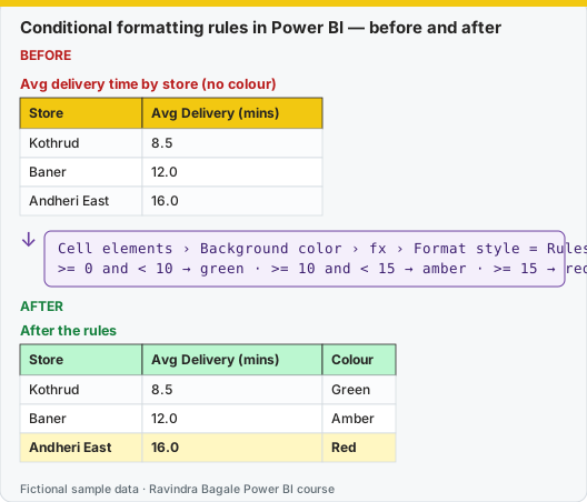
Same before / after tables as text
Before — Avg delivery time by store (no colour)
| Store | Avg Delivery (mins) |
|---|---|
| Kothrud | 8.5 |
| Baner | 12.0 |
| Andheri East | 16.0 |
Formula / click path
Cell elements › Background color › fx › Format style = Rules
>= 0 and < 10 → green · >= 10 and < 15 → amber · >= 15 → red
After — After the rules
| Store | Avg Delivery (mins) | Colour |
|---|---|---|
| Kothrud | 8.5 | Green |
| Baner | 12.0 | Amber |
| Andheri East | 16.0 | Red |
Do it step by step:
- Build a table: Store Name and Avg Delivery Time (mins).
- Open Format › Cell elements. Pick the delivery column in Apply settings to.
- Turn on Background color. Click fx.
- Format style: Rules. Add three rules: 0 to 10 green, 10 to 15 amber, 15 and above red.
- In the last rule, use a high upper number such as 999, so no value falls through.
- Click OK. Check: Andheri East is red. Remember, here a low number is good.
एक-एक step करून बघा:
- Table बनवा: Store Name आणि Avg Delivery Time (mins).
- Format › Cell elements उघडा. Apply settings to मध्ये delivery column निवडा.
- Background color चालू करा. fx वर click करा.
- Format style: Rules. तीन rules जोडा: 0 ते 10 हिरवा, 10 ते 15 amber, 15 आणि वर लाल.
- शेवटच्या rule मध्ये 999 सारखा मोठा वरचा number वापरा, म्हणजे कोणतीही value सुटत नाही.
- OK करा. तपासा: Andheri East लाल आहे. लक्षात ठेवा, इथे कमी number चांगला.
एक-एक step करके देखिए:
- Table बनाइए: Store Name और Avg Delivery Time (mins).
- Format › Cell elements खोलिए. Apply settings to में delivery column चुनिए.
- Background color चालू कीजिए. fx पर click कीजिए.
- Format style: Rules. तीन rules जोड़िए: 0 से 10 हरा, 10 से 15 amber, 15 और ऊपर लाल.
- आख़िरी rule में 999 जैसा बड़ा ऊपरी number इस्तेमाल कीजिए, ताकि कोई value न छूटे.
- OK कीजिए. जाँचिए: Andheri East लाल है. याद रखिए, यहाँ कम number अच्छा है.
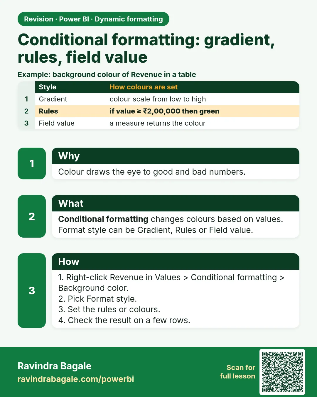
Conditional formatting changes colours or icons based on values. There are three format styles:
| Format style | How it works | Example |
|---|---|---|
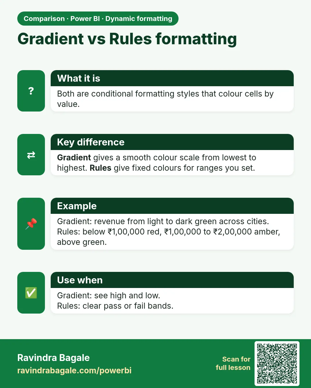
| Gradient (colour scale) | Lowest value → one colour, highest → another (optional middle colour) | Avg Delivery Time: green (low) → yellow → red (high) |
| Rules | If value is in a range, then use a colour | ≤ 10 green, > 10 and ≤ 15 amber, > 15 red |
| Field value | A column or measure returns the colour (name or hex code like #D13438) |
A DAX colour measure (reusable everywhere) |
The DAX colour measure (field value):
Delivery Time Colour =
VAR t = [Avg Delivery Time (mins)]
RETURN
SWITCH(TRUE(),
    ISBLANK(t), BLANK(),
    t <= 10, "#107C10",     -- green
    t <= 15, "#F2A900",     -- amber
    "#D13438")              -- red: slower than 15 minutes
Steps in Power BI – colour the Avg Delivery Time column in a table
- Build a table: Store Name, Total Orders, Avg Delivery Time (mins), Cancellation Rate.
- In Build visual, click the drop-down arrow on Avg Delivery Time (mins) in Columns › Conditional formatting › Background color. (Or Format visual › Visual › Cell elements › Apply settings to the column › Background color On › fx.)
- Format style: Rules. Apply to: Values only. What field should we base this on?: Avg Delivery Time (mins). Summarization: (measure).
- Rules: If value ≥ 0 Number and ≤ 10 Number then green; > 10 and ≤ 15 amber; > 15 and ≤ 999 red. Click + New rule for each › OK.
- Or choose Format style Field value ›
[Delivery Time Colour]› OK. The same colours are now controlled by one measure. - Font color: use white font for the red cells with another field-value measure.
Empty values
In the Gradient dialog, How should we format empty values? lets you choose how blanks are shown (for example Don't format or a specific colour). Cancelled-only stores with no delivery time will not look "perfect green".
Conditional formatting makes the report "speak". But do not use too many colours – highlight only what matters.
Conditional formatting ने report "बोलतो". पण रंग जास्त वापरू नका – फक्त महत्त्वाचं highlight करा.
Conditional formatting से report "बोलती" है. पर रंग ज़्यादा मत इस्तेमाल कीजिए – सिर्फ़ ज़रूरी चीज़ highlight कीजिए.
Ravindra Bagale's Tip
Friends, many students use a colour gradient on a measure where low is good (delivery time) with green at the high end. Check the direction of every colour rule, or drive the colour from a measure that returns a colour name or hex code based on business thresholds. This matters for both exams and interviews.
Ravindra Bagale's Tip – मराठी
मित्रांनो, बरेच students कमी value चांगली असलेल्या measure वर (delivery time) हिरवा रंग वरच्या टोकाला ठेवून colour gradient वापरतात. प्रत्येक colour rule ची दिशा चेक करा, किंवा business thresholds वर आधारित colour name किंवा hex code देणाऱ्या measure ने रंग ठरवा. हे exam आणि interview दोन्हीसाठी important आहे.
Ravindra Bagale's Tip – हिंदी
दोस्तों, बहुत से students ऐसे measure पर जहाँ कम value अच्छी है (delivery time) हरे रंग को ऊँचे सिरे पर रखकर colour gradient लगाते हैं. हर colour rule की दिशा check करो, या business thresholds के आधार पर colour name या hex code देने वाले measure से रंग तय करो. यह exam और interview दोनों के लिए ज़रूरी है.
Fix common mistakes
| Wrong result | Reason | Correction |
|---|---|---|
| All rows red | Rule typed as 50 instead of 0.5 | Use decimals, or choose Percent in the rule |
| Total row coloured | Apply to totals on | Choose Values only |
| Colour-only meaning | Colour-blind readers | Add an icon or the word Below |
Practise independently
Practice task
Change the target rule to 30%. Which cities are red?
Hints
- Compare with 0.3.
Solution
None – all are ≥ 33.3%.
Think like a professional
Thresholds belong to the business. Store them in a table or measure so they can change without editing visuals.
 Revision card
 Comparison card