Labs · Power BI
Lab: Glossary Match-Up – 25 Power BI Terms with Your Own One-Line Examples
Course: Power BI · Chapter 33: Glossary
Chapter 33 is the glossary; this lab makes you match the terms and tie each one to something you built.
Download powerbi_glossary_25.csv (25 terms, shuffled meanings)
Chala mitrano! A glossary read once is forgotten in a week. A glossary you match yourself, with an example from your own work, stays. Today: 25 terms, 25 shuffled meanings, one score, and then the important part: your own one-line example for each. Shabda tumche, udaharan tumche!
चला मित्रांनो! एकदा वाचलेली glossary आठवड्यात विसरते. स्वतः match केलेली, स्वतःच्या कामातलं उदाहरण दिलेली glossary लक्षात राहते. आज: 25 terms, 25 shuffled meanings, एक score, आणि मग महत्त्वाचा भाग: प्रत्येकासाठी तुमचं स्वतःचं एका ओळीचं उदाहरण. शब्द तुमचे, उदाहरण तुमचे!
चलो दोस्तों! एक बार पढ़ी glossary हफ्ते में भूल जाती है। खुद match की हुई, अपने काम के उदाहरण वाली glossary याद रहती है। आज: 25 terms, 25 shuffled meanings, एक score, और फिर ज़रूरी हिस्सा: हर term के लिए आपका अपना एक लाइन का उदाहरण। शब्द आपके, उदाहरण आपके!
Suppose we are…
Suppose we have joined Wipro as a trainee and the first weekly test is a Power BI vocabulary round: the trainer reads a term like "gateway" or "filter context" and we must explain it in one line with an example. We will practise with a spreadsheet of 25 terms and 25 meanings in shuffled order (letters A to Y).
Goal of this lab
- Match all 25 terms to their meanings without notes (10 minutes).
- Score yourself with one formula.
- Write a one-line example from your own labs for each term.
What you need (all free)
- Google Sheets, Excel or LibreOffice Calc.
- Download powerbi_glossary_25.csv (25 terms, shuffled meanings)
- 30 minutes and no notes for the first 10.
The data: before and after
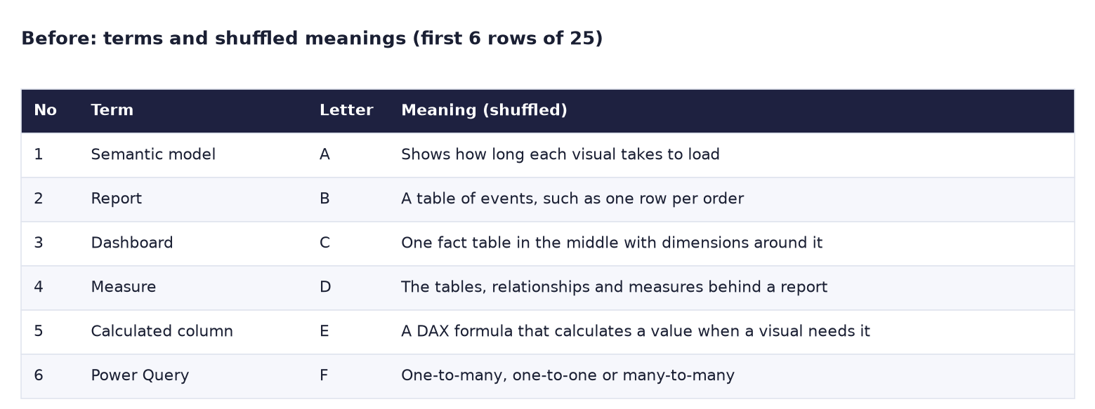
Before. Terms on the left, meanings shuffled on the right with letters A–Y. The "Your letter" and "Your one-line example" columns are empty.
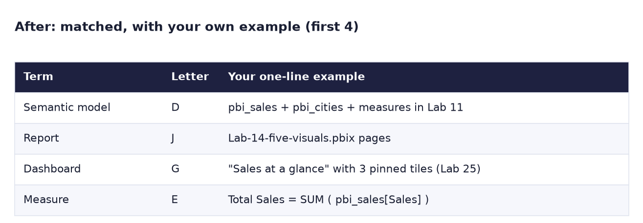
After. Each term has the right letter and an example from your own work.
The formula
To score yourself, type the answer key into column G (rows 2–26) after you finish, then in any empty cell:
=SUMPRODUCT(--(UPPER(TRIM(C2:C26))=G2:G26))
C2:C26is your letters;G2:G26is the key.TRIMandUPPERforgive a stray space or a small letter.--( … )turns TRUE/FALSE into 1/0, andSUMPRODUCTadds them up: your score out of 25.
To see which ones you got wrong, put this in H2 and fill down: =IF(UPPER(TRIM(C2))=G2,"OK","CHECK").
Steps
-
Open the CSV in Google Sheets (File → Import → Upload, "Replace spreadsheet") or in Excel/Calc.
What you should see: 26 rows (1 header + 25 terms) and 6 columns: No, Term, Your letter, Your one-line example, Letter, Meaning (shuffled).
-
Start a 10-minute timer. For each term in column B, read the meanings in column F and type the matching letter in column C. Each letter is used exactly once.
- When the timer ends, stop, even if some are empty.
-
Open the answer key below and type it into G2:G26.
Answer key (open only after the timer)
1-D, 2-J, 3-G, 4-E, 5-K, 6-X, 7-H, 8-V, 9-U, 10-B, 11-P, 12-C, 13-L, 14-F, 15-I, 16-T, 17-R, 18-S, 19-Y, 20-O, 21-W, 22-M, 23-N, 24-Q, 25-A
-
Type the SUMPRODUCT formula in an empty cell (for example I1) and the check formula in H2, filled down to H26.
What you should see: a number out of 25 in I1, and "OK" or "CHECK" next to each term. 20 or more is good for now.
-
For every "CHECK" row, read the right meaning and say it aloud once.
- Now fill column D for all 25 terms with your own one-line example. Use what you built: for example, Star schema → "pbi_sales in the middle with DateTable, pbi_products and pbi_cities (Lab 11)"; RLS → "Pune manager sees only Pune, 346,000 (Lab 26)".
- Save the sheet. Before an interview, read only columns B and D.
Ravindra Bagale's Tip
Watch the pairs that students mix up: Report vs Dashboard, Measure vs Calculated column, Import vs DirectQuery, Power Query vs DAX. For each pair, write one sentence with "but": "A report can have many pages, but a dashboard is one page of pinned tiles in the Service." Jodi samjli, gondhal sampla!
Ravindra Bagale's Tip – मराठी
Students ज्या जोड्या गोंधळतात त्या लक्षात ठेवा: Report vs Dashboard, Measure vs Calculated column, Import vs DirectQuery, Power Query vs DAX. प्रत्येक जोडीसाठी "पण" वापरून एक वाक्य लिहा: "Report ला अनेक pages असू शकतात, पण dashboard हे Service मधलं pinned tiles चं एक page असतं." जोडी समजली, गोंधळ संपला!
Ravindra Bagale's Tip – हिंदी
Students जो जोड़ियाँ गड़बड़ाते हैं उन पर ध्यान दो: Report vs Dashboard, Measure vs Calculated column, Import vs DirectQuery, Power Query vs DAX। हर जोड़ी के लिए "लेकिन" वाला एक वाक्य लिखो: "Report में कई pages हो सकते हैं, लेकिन dashboard, Service में pinned tiles का एक page होता है।" जोड़ी समझी, गड़बड़ खत्म!
Common mistakes
| Mistake | What happens | Fix |
|---|---|---|
| Opening the CSV by double-click in Excel with odd regional settings | Meanings with commas split into extra columns | Use Data → From Text/CSV, or Google Sheets import |
| Typing "d " or "d" | The formula marks a right answer wrong | UPPER(TRIM( … )) in the formula |
| Peeking at the key early | A high score you cannot repeat | Timer first, key after |
| Copying the meaning as the example | Column D adds nothing | Example = something you built, with a name or number |
| Mixing up Report and Dashboard | A classic interview slip | Dashboard = Service only, one page, pinned tiles |
Self-check checklist
0 of 5 done
Try-at-home challenge
Add 5 more terms of your own to rows 27–31 (for example: Tooltip page, Sync slicers, Mark as date table, Workspace, Scheduled refresh). Write the meaning and your example. Then extend the score formula so it counts all 30 terms.
Check your answer
Sample meanings: Tooltip page = a small report page shown when you hover over a data point (Lab 18); Sync slicers = the same slicer selection applied on several pages (Lab 22); Mark as date table = tells Power BI which table and Date column to use for time intelligence (Lab 11); Workspace = a container in the Service for reports, models and dashboards (Lab 25); Scheduled refresh = the Service refreshing the data at set times (Lab 25). The formula becomes =SUMPRODUCT(--(UPPER(TRIM(C2:C31))=G2:G31)), out of 30.
Samjla ka? Match first, score with one formula, then tie every term to your own work. Aata pudhe jaauya: plan a real project from a client brief.