Excel Interview Prep — Intermediate

By Ravindra Bagale · Last updated: 31 October 2026

Friends, intermediate round: IFS, date SUMIFS, INDEX-MATCH, Pivot vs helper, CF formulas and clean Power Query steps. Speak the why, then type the formula.

Fictional sample data for learning. Industry flavour: Regional retail MIS (Pune / Birmingham / Dubai) with ₹ / £ / AED. Brands and people are made up for practice.

Why → What → How

Why: Excel interviews are not memory tests of every function name. They check if you can clean a small sheet, write a correct formula, and explain the result in plain English.

What: This page has 28 real interview-style questions for Intermediate. Each one has a short answer, vertical steps, a tiny example, a common wrong answer, and a follow-up question.

How — study plan:

Skim all question titles once (10 minutes).
Download the practice workbook and open sheet About this data.
Answer aloud, then type the formula in the file.
Check the yellow cells on sheet Answers only after you try.
Revise with the three cards and take the quiz.

Download practice file: practice-intermediate-interview.xlsx (includes About this data, practice sheets, Answers).

Ravindra Bagale's Tip

Friends, when SUM after Filter looks wrong, switch to SUBTOTAL — that one interview trap catches many people.

Ravindra Bagale's Tip

Prefer a helper column you can audit over a magic Pivot calculated field you cannot see in the sheet.

Questions (28)

Q1 · Formula

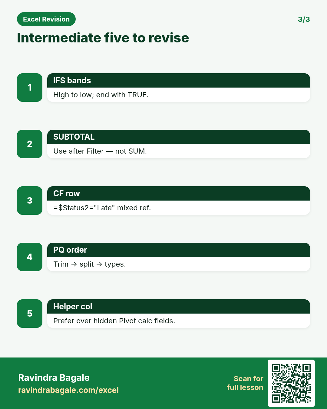
When do you use IFS instead of nested IF?

Why interviewers ask: To see if you understand the idea, not only the button clicks.

What (short answer): IFS checks many conditions in order and returns the first match. It is easier to read than nested IF for grade bands.

How — tiny example (vertical steps):

Marks in B2=78.
Write =IFS(B2>=75,"A",B2>=60,"B",B2>=35,"C",TRUE,"F").
Result A. Change to 50 → C.

Formula: =IFS(B2>=75,"A",B2>=60,"B",B2>=35,"C",TRUE,"F")
Result: A
What it means: Grade band without nested IF.

Common wrong answer: Writing overlapping conditions in the wrong order (60 before 75).

Follow-up they often ask: How do you handle a blank marks cell?

Q2 · Formula

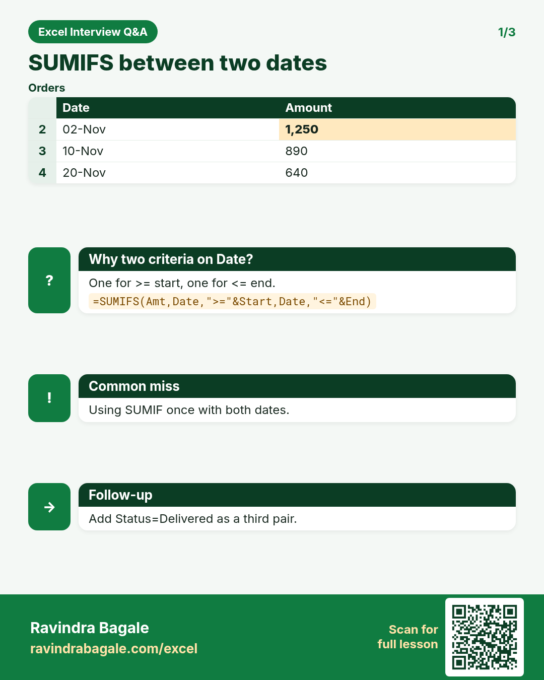
Write SUMIFS for sales between two dates.

Why interviewers ask: To see if you understand the idea, not only the button clicks.

What (short answer): SUMIFS can use >= start and <= end on the same date column as two criteria pairs.

How — tiny example (vertical steps):

Dates in A, Amount in B. Start in E1, End in E2.
=SUMIFS(B:B,A:A,">="&E1,A:A,"<="&E2).
Only rows inside the window are added.

Formula: =SUMIFS(B2:B100,A2:A100,">="&E1,A2:A100,"<="&E2)
Result: window total
What it means: Month or week sales.

Common wrong answer: Using SUMIF once with both dates (SUMIF takes only one condition).

Follow-up they often ask: How do you exclude Cancelled in the same formula?

Q3 · Formula

Explain approximate VLOOKUP for tax slabs.

Why interviewers ask: To see if you understand the idea, not only the button clicks.

What (short answer): With range_lookup TRUE, VLOOKUP finds the largest value less than or equal to the lookup value in a sorted first column — perfect for slabs.

How — tiny example (vertical steps):

Slab table: 0→5%, 50000→10%, 100000→15% sorted ascending.
Income 72000. =VLOOKUP(72000,slabs,2,TRUE) → 10%.

Formula: =VLOOKUP(72000,$E$2:$F$4,2,TRUE)
Result: 10%
What it means: Income falls in the 50k slab.

Common wrong answer: Using FALSE and getting #N/A because 72000 is not an exact key.

Follow-up they often ask: What happens if the slab table is not sorted?

Q4 · Formula

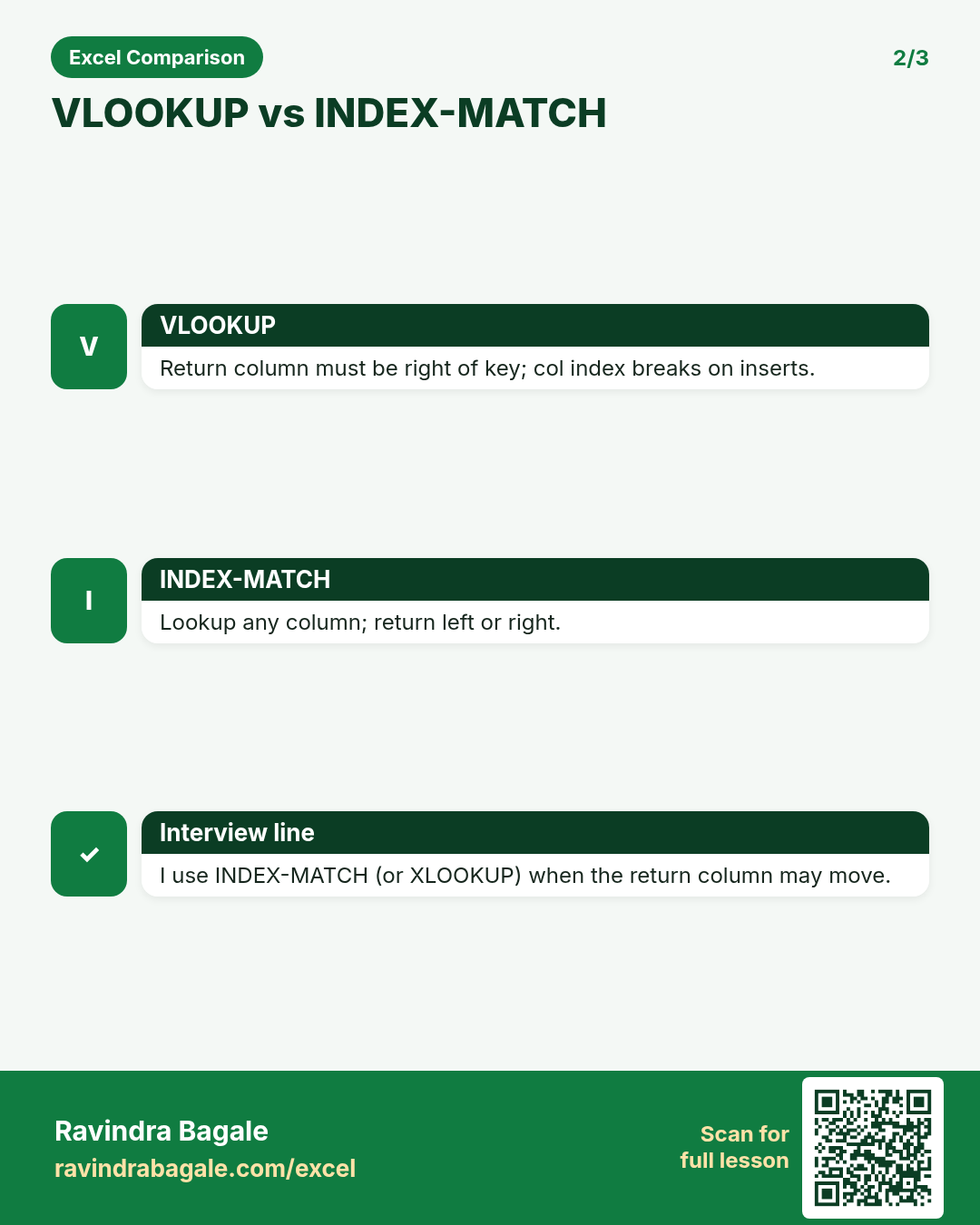
How is INDEX-MATCH different from VLOOKUP?

Why interviewers ask: To see if you understand the idea, not only the button clicks.

What (short answer): INDEX-MATCH looks up a value in any column and returns from any other column (left or right). Column inserts do not break the column index the same way.

How — tiny example (vertical steps):

Names in B, IDs in A. Find ID for "Aisha Khan".
=INDEX(A:A,MATCH("Aisha Khan",B:B,0)).

Formula: =INDEX(A2:A50,MATCH("Aisha Khan",B2:B50,0))
Result: EMP-104
What it means: ID looked up from name on the right of ID.

Common wrong answer: Saying INDEX-MATCH is always faster — focus on flexibility first.

Follow-up they often ask: How do you do a two-way INDEX-MATCH (row and column)?

Q5 · Theory

Pivot calculated field vs helper column — which first?

Why interviewers ask: To see if you understand the idea, not only the button clicks.

What (short answer): Prefer a helper column in the source table when the logic is reusable and auditable. Use a Pivot calculated field only for quick Pivot-only maths.

How — tiny example (vertical steps):

Need Profit = Amount-Cost.
Add Profit column in the Table with =[@Amount]-[@Cost].
Pivot on Profit. Avoid hiding logic only inside Pivot.

Formula: =[@Amount]-[@Cost]
Result: helper Profit
What it means: Clear audit trail in the Table.

Common wrong answer: Building five calculated fields that nobody can see in the sheet.

Follow-up they often ask: Can a calculated field use COUNTIF?

Q6 · Theory

How do you build dependent drop-downs?

Why interviewers ask: To see if you understand the idea, not only the button clicks.

What (short answer): Data Validation on the first list (Region). Second list uses INDIRECT or FILTER based on the region cell so only related cities appear.

How — tiny example (vertical steps):

Name ranges WestCities, EastCities.
City cell validation: =INDIRECT(A2&"Cities") where A2 is West/East.

Formula: =INDIRECT(A2&"Cities")
Result: city list
What it means: City choices follow region.

Common wrong answer: Hard-coding one city list for all regions.

Follow-up they often ask: How do you avoid INDIRECT with FILTER in Microsoft 365?

Q7 · Formula

Highlight an entire row with conditional formatting formula.

Why interviewers ask: To see if you understand the idea, not only the button clicks.

What (short answer): Use a formula with a mixed reference that locks the column of the status test, applied to the full row range.

How — tiny example (vertical steps):

Select A2:F100. Home → Conditional Formatting → New Rule → Formula.
=$E2="Late" (lock column E).
Pick a red fill.

Formula: =$E2="Late"
Result: row turns red
What it means: Late rows stand out in a tracker.

Common wrong answer: Using =E2="Late" without $ so only one column highlights.

Follow-up they often ask: How do you stop CF when the row is blank?

Q8 · Theory

Flash Fill vs formulas — when each?

Why interviewers ask: To see if you understand the idea, not only the button clicks.

What (short answer): Flash Fill (Ctrl+E) is fast for one-off patterns. Formulas (LEFT/TEXTBEFORE) stay live when source data changes.

How — tiny example (vertical steps):

Split "Priya Sharma" once with Flash Fill.
If new rows arrive daily, use =TEXTBEFORE(A2," ") instead.

Formula: Ctrl+E
Result: split names
What it means: One-time clean vs live formula.

Common wrong answer: Relying on Flash Fill inside a monthly refresh pack.

Follow-up they often ask: Does Flash Fill work on protected sheets?

Q9 · Theory

How do you remove duplicates safely?

Why interviewers ask: To see if you understand the idea, not only the button clicks.

What (short answer): First copy the sheet or take a backup. Then Data → Remove Duplicates on the key columns. Or use UNIQUE to spill a clean list without destroying the source.

How — tiny example (vertical steps):

Backup sheet.
Select Table → Data → Remove Duplicates → tick OrderID.
Or =UNIQUE(A2:A500) on a new sheet.

Formula: =UNIQUE(A2:A500)
Result: unique IDs
What it means: Safe dedupe view.

Common wrong answer: Removing duplicates on the only copy with the wrong columns ticked.

Follow-up they often ask: How do you keep the latest row per ID?

Q10 · Theory

When is a dual-axis chart useful?

Why interviewers ask: To see if you understand the idea, not only the button clicks.

What (short answer): When two series have very different scales (₹ sales vs % margin). Use sparingly — label axes clearly so people are not misled.

How — tiny example (vertical steps):

Combo chart: columns for Sales, line for Margin %.
Format Margin series → Secondary axis.
Title both axes.

Formula: (Combo chart)
Result: two scales
What it means: Sales and margin together.

Common wrong answer: Putting unrelated metrics on two axes to force a story.

Follow-up they often ask: What is a better alternative for many KPIs?

Q11 · Formula

What does TEXTJOIN do that & cannot easily do?

Why interviewers ask: To see if you understand the idea, not only the button clicks.

What (short answer): TEXTJOIN adds a delimiter between many cells and can ignore blanks.

How — tiny example (vertical steps):

A2:A4 = Red, (blank), Blue.
=TEXTJOIN(", ",TRUE,A2:A4) → Red, Blue.

Formula: =TEXTJOIN(", ",TRUE,A2:A4)
Result: Red, Blue
What it means: Clean list skipping blanks.

Common wrong answer: Using CONCAT and getting double commas for blanks.

Follow-up they often ask: How is TEXTJOIN different from TEXTSPLIT?

Q12 · Formula

NETWORKDAYS vs a simple date subtraction?

Why interviewers ask: To see if you understand the idea, not only the button clicks.

What (short answer): NETWORKDAYS counts working days between two dates and can skip a holiday list. Subtraction counts all calendar days.

How — tiny example (vertical steps):

Start 3-Nov-2026, End 10-Nov-2026.
=NETWORKDAYS(start,end) skips weekends.

Formula: =NETWORKDAYS(A2,B2,$H$2:$H$10)
Result: working days
What it means: SLA in business days.

Common wrong answer: Using =B2-A2 for a vendor SLA that excludes Sundays.

Follow-up they often ask: What does NETWORKDAYS.INTL add?

Q13 · Formula

SUBTOTAL vs SUM on a filtered list?

Why interviewers ask: To see if you understand the idea, not only the button clicks.

What (short answer): SUBTOTAL (and AGGREGATE) can ignore hidden filtered rows. SUM always includes hidden rows.

How — tiny example (vertical steps):

Filter City=Pune.
=SUM(Amount) still totals all cities.
=SUBTOTAL(9,Amount) totals only visible Pune rows.

Formula: =SUBTOTAL(9,D2:D200)
Result: visible total
What it means: Correct total after Filter.

Common wrong answer: Reporting SUM after Filter and getting a surprise grand total.

Follow-up they often ask: What function number is AVERAGE in SUBTOTAL?

Q14 · Theory

What is an Excel Table slicer?

Why interviewers ask: To see if you understand the idea, not only the button clicks.

What (short answer): A slicer is a clickable filter button for an Excel Table or PivotTable. It makes filtering obvious for non-Excel users.

How — tiny example (vertical steps):

Click inside Table → Table Design → Insert Slicer → City.
Click Pune — rows filter.

Formula: (Insert Slicer)
Result: filter buttons
What it means: Friendly filter UI.

Common wrong answer: Thinking slicers work only on PivotTables (Tables support them too in modern Excel).

Follow-up they often ask: Can one slicer drive two PivotTables?

Q15 · Theory

What is Goal Seek in one sentence?

Why interviewers ask: To see if you understand the idea, not only the button clicks.

What (short answer): Goal Seek changes one input cell until a formula cell reaches the value you want.

How — tiny example (vertical steps):

Want EMI cell = 25000 by changing loan amount.
Data → What-If → Goal Seek.
Set cell EMI to 25000 by changing Loan.

Formula: Goal Seek
Result: input found
What it means: Reverse calculation.

Common wrong answer: Using Goal Seek when two inputs must change (use Solver).

Follow-up they often ask: Does Goal Seek keep a history of tries?

Q16 · Formula

Named ranges — why bother?

Why interviewers ask: To see if you understand the idea, not only the button clicks.

What (short answer): A name like TaxRate is easier to read than $H$1 and reduces mistakes when sharing files.

How — tiny example (vertical steps):

Select H1 → Name Box type TaxRate → Enter.
Formula =Amount*TaxRate.

Formula: =B2*TaxRate
Result: GST amount
What it means: Readable formula.

Common wrong answer: Creating names that look like cell addresses (A1 style confusion).

Follow-up they often ask: How do you see all names in a workbook?

Q17 · Theory

Sheet protection vs workbook protection?

Why interviewers ask: To see if you understand the idea, not only the button clicks.

What (short answer): Sheet protection locks cells on one sheet. Workbook protection locks structure (add/delete/move sheets). Different passwords and purposes.

How — tiny example (vertical steps):

Unlock input cells (Format Cells → Protection → untick Locked).
Review → Protect Sheet.
Review → Protect Workbook for structure.

Formula: (Protect Sheet)
Result: inputs editable
What it means: Users can type only where allowed.

Common wrong answer: Protecting the sheet with every cell locked including inputs.

Follow-up they often ask: Can users still copy values out of a protected sheet?

Q18 · Theory

Power Query first clean: split, trim, types — order?

Why interviewers ask: To see if you understand the idea, not only the button clicks.

What (short answer): Get Data → trim text → split columns → set data types → remove duplicates → Close & Load. Order matters because types affect splits.

How — tiny example (vertical steps):

Home → Trim.
Split Column by Delimiter.
Change Type to Date/Decimal.

Formula: (Power Query)
Result: clean query
What it means: Refreshable clean steps.

Common wrong answer: Changing type to Whole Number before trimming spaces that block conversion.

Follow-up they often ask: Where are the Applied Steps kept?

Q19 · Formula

COUNTIFS with three conditions — example.

Why interviewers ask: To see if you understand the idea, not only the button clicks.

What (short answer): COUNTIFS counts rows that pass every criteria pair.

How — tiny example (vertical steps):

Count Delivered Snacks in Pune.
=COUNTIFS(City,"Pune",Category,"Snacks",Status,"Delivered").

Formula: =COUNTIFS(C:C,"Pune",E:E,"Snacks",I:I,"Delivered")
Result: count
What it means: Multi-filter count.

Common wrong answer: Nesting COUNTIF inside COUNTIF.

Follow-up they often ask: How do you count unique cities?

Q20 · Scenario

Manager asks: top 3 cities by sales this month. Steps?

Why interviewers ask: To see if you understand the idea, not only the button clicks.

What (short answer): Filter or Pivot by month, summarise sales by city, sort descending, take top 3. Or use SORT+TAKE in Microsoft 365.

How — tiny example (vertical steps):

Pivot: City rows, Sum of Amount, filter Month.
Sort values Z→A.
Read first three cities.

Formula: =TAKE(SORT(city_sales,2,-1),3)
Result: top 3
What it means: Leaderboard answer.

Common wrong answer: Sorting the raw transaction sheet without aggregating first.

Follow-up they often ask: How do you break ties?

Q21 · Practical

On the practice sheet, build a Pivot: City × Status with Amount.

Why interviewers ask: To see if you understand the idea, not only the button clicks.

What (short answer): Insert PivotTable, put City on Rows, Status on Columns, Amount in Values as Sum.

How — tiny example (vertical steps):

Select Orders table.
Insert → PivotTable.
Arrange fields as above.

Formula: (PivotTable)
Result: matrix
What it means: City and status sales.

Common wrong answer: Putting Amount on Rows instead of Values.

Follow-up they often ask: How do you show % of Grand Total?

Q22 · Formula

XLOOKUP exact match basic syntax?

Why interviewers ask: To see if you understand the idea, not only the button clicks.

What (short answer): XLOOKUP(lookup_value, lookup_array, return_array). Default is exact match. Can search right-to-left.

How — tiny example (vertical steps):

=XLOOKUP("Pune",City,Manager) returns the manager name.

Formula: =XLOOKUP(G2,A:A,B:B)
Result: manager
What it means: Modern lookup.

Common wrong answer: Still teaching only VLOOKUP when XLOOKUP is available.

Follow-up they often ask: What does if_not_found do?

Q23 · Theory

Data Validation error alert — why set it?

Why interviewers ask: To see if you understand the idea, not only the button clicks.

What (short answer): It stops bad inputs (wrong date, text in qty) and shows a clear message so MIS stays clean.

How — tiny example (vertical steps):

Data → Data Validation → Whole number >=1.
Error Alert: Stop + message "Qty must be 1+".

Formula: (Data Validation)
Result: bad input blocked
What it means: Cleaner source data.

Common wrong answer: Using only Input Message without Error Alert (users can still type junk).

Follow-up they often ask: Warning vs Stop style?

Q24 · Formula

AVERAGEIFS example for delivered minutes in one city.

Why interviewers ask: To see if you understand the idea, not only the button clicks.

What (short answer): AVERAGEIFS averages a range with multiple filters.

How — tiny example (vertical steps):

=AVERAGEIFS(Mins,City,"Nashik",Status,"Delivered").

Formula: =AVERAGEIFS(H:H,C:C,"Nashik",I:I,"Delivered")
Result: avg mins
What it means: City SLA.

Common wrong answer: Averaging after a Filter with AVERAGE (includes hidden).

Follow-up they often ask: How do you ignore zeros?

Q25 · Scenario

VLOOKUP returns #N/A — name your debug checklist.

Why interviewers ask: To see if you understand the idea, not only the button clicks.

What (short answer): Check exact spelling, TRIM spaces, number vs text IDs, correct column index, range_lookup FALSE, and whether the key exists.

How — tiny example (vertical steps):

=TRIM both sides.
Check =A2=G2 for TRUE.
Confirm col_index_num.

Formula: =IFNA(VLOOKUP(...),"Missing")
Result: friendly miss
What it means: Debugged lookup.

Common wrong answer: Changing data until #N/A disappears without understanding why.

Follow-up they often ask: How do you find which keys are missing with MATCH?

Q26 · Practical

Create a named Table and a total row for Amount.

Why interviewers ask: To see if you understand the idea, not only the button clicks.

What (short answer): Ctrl+T → check headers → Table Design → Total Row → Amount = Sum.

How — tiny example (vertical steps):

Select data → Ctrl+T.
Enable Total Row.
Choose Sum on Amount.

Formula: Ctrl+T
Result: Table + total
What it means: Structured references ready.

Common wrong answer: Leaving a blank row inside the range so Ctrl+T stops early.

Follow-up they often ask: How do you add a calculated column?

Q27 · Formula

Explain IFERROR wrapping a lookup.

Why interviewers ask: To see if you understand the idea, not only the button clicks.

What (short answer): IFERROR returns a fallback when the formula errors. Prefer IFNA when you only want to catch #N/A.

How — tiny example (vertical steps):

=IFERROR(VLOOKUP(G2,A:B,2,FALSE),"Not found").

Formula: =IFERROR(VLOOKUP(G2,A:B,2,FALSE),"Not found")
Result: Not found
What it means: Clean output.

Common wrong answer: Wrapping everything in IFERROR and hiding real #DIV/0! bugs.

Follow-up they often ask: IFNA vs IFERROR?

Q28 · Theory

How do you document a workbook for the next person?

Why interviewers ask: To see if you understand the idea, not only the button clicks.

What (short answer): About sheet, named ranges list, colour inputs yellow, lock formulas, short README of refresh steps.

How — tiny example (vertical steps):

Add About this data sheet.
Yellow = inputs.
Protect formula cells.

Formula: (About sheet)
Result: handover ready
What it means: MIS discipline.

Common wrong answer: Leaving only passwords and no explanation.

Follow-up they often ask: What belongs in a KPI dictionary sheet?

Practice tasks (12)

1. IFS grades for Marks!B (easy)
Hint: Order bands from high to low; end with TRUE.
2. SUMIFS for 1–15 Nov window (medium)
Hint: Two criteria on the same date column.
3. Approximate VLOOKUP fee slab (medium)
Hint: Sort slabs ascending; range_lookup TRUE.
4. INDEX-MATCH id from name (medium)
Hint: MATCH finds the row; INDEX returns the column.
5. CF entire row when Status=Late (medium)
Hint: Mixed reference on the status column.
6. Dependent city drop-down (hard)
Hint: Named ranges + INDIRECT or FILTER.
7. SUBTOTAL under a City filter (easy)
Hint: Function number 9 is SUM.
8. NETWORKDAYS with holiday list (medium)
Hint: Third argument is the holiday range.
9. Pivot City × Status Amount (medium)
Hint: Amount goes in Values as Sum.
10. XLOOKUP manager by city (easy)
Hint: lookup_array then return_array.
11. Trim + unique city list (medium)
Hint: TRIM helper then UNIQUE.
12. Document About this data (easy)
Hint: Say what each row and column means.

Quiz (8 questions)

Interview, comparison and revision cards

Standalone cards (no tip or photo strip). Each has a QR to this lesson. Download the PNG and revise offline.

Interview card SUMIFS dates — Interview card 1/3 — SUMIFS dates

Comparison VLOOKUP vs INDEX-MATCH — Comparison card 2/3 — VLOOKUP vs INDEX-MATCH

Revision intermediate five — Revision card 3/3 — Intermediate five

Next: back to the Interview Prep hub · related lesson Formulas and Functions.