Excel Interview Prep — Data Analyst
Friends, analyst interview mode: SUMIFS, XLOOKUP, FILTER, Pivot, Power Query, KPIs and debugging wrong totals. Easy English, real scenarios, practice file included.
चला मित्रांनो — analyst interview: SUMIFS, XLOOKUP, FILTER, Pivot, Power Query, KPIs आणि चुकीचे totals. सोपी भाषा, खास scenarios, practice file.
चलो दोस्तों — analyst interview: SUMIFS, XLOOKUP, FILTER, Pivot, Power Query, KPIs और गलत totals. सरल भाषा, असली scenarios, practice file.
Why → What → How
Why: Excel interviews are not memory tests of every function name. They check if you can clean a small sheet, write a correct formula, and explain the result in plain English.
What: This page has 32 real interview-style questions for Data Analyst. Each one has a short answer, vertical steps, a tiny example, a common wrong answer, and a follow-up question.
How — study plan:
- Skim all question titles once (10 minutes).
- Download the practice workbook and open sheet
About this data. - Answer aloud, then type the formula in the file.
- Check the yellow cells on sheet
Answersonly after you try. - Revise with the three cards and take the quiz.
Download practice file: practice-data-analyst-interview.xlsx (includes About this data, practice sheets, Answers).
Ravindra Bagale's Tip
Friends, in analyst interviews they care about SUMIFS, XLOOKUP, Pivot, Power Query and how you define a KPI. Speak definitions before formulas.
Ravindra Bagale's Tip – मराठी
मित्रांनो, analyst interview मध्ये SUMIFS, XLOOKUP, Pivot, Power Query आणि KPI definition महत्त्वाची. आधी definition, मग formula.
Ravindra Bagale's Tip – हिंदी
दोस्तों, analyst interview में SUMIFS, XLOOKUP, Pivot, Power Query और KPI definition मायने रखते हैं. पहले definition, फिर formula.
Ravindra Bagale's Tip
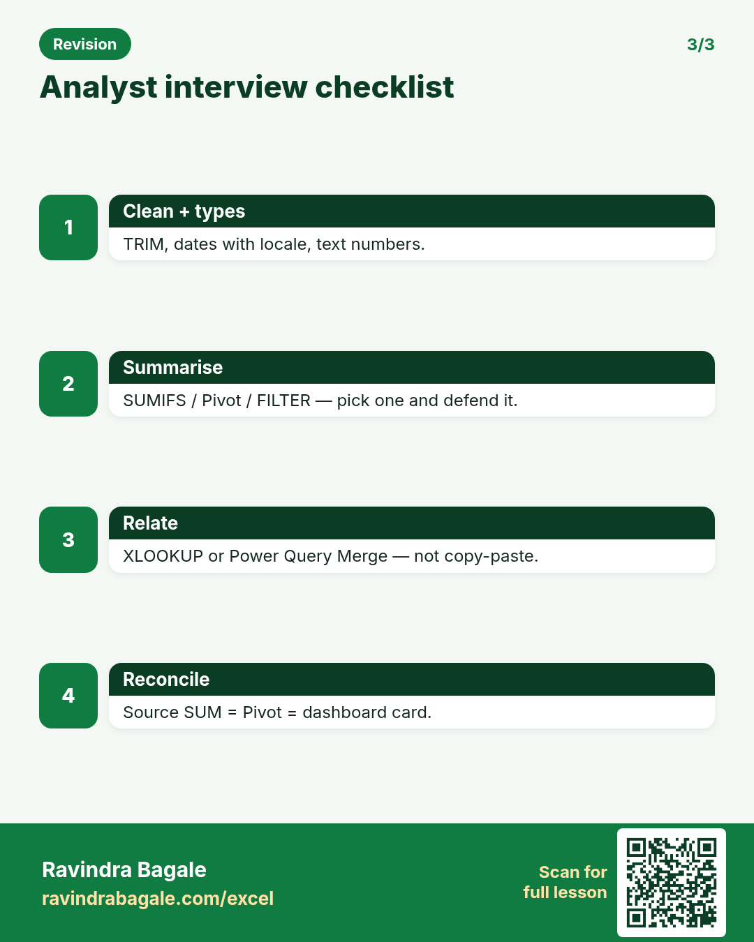
When totals disagree, do not argue — reconcile. Source SUM vs Pivot grand total vs dashboard card, then check filters.
Ravindra Bagale's Tip – मराठी
Totals जुळत नसतील तर भांडू नका — reconcile करा. Source SUM, Pivot total, dashboard card, मग filters.
Ravindra Bagale's Tip – हिंदी
Totals न जुड़ें तो बहस नहीं — reconcile करो. Source SUM, Pivot total, dashboard card, फिर filters.
Questions (32)
What does a data analyst do with Excel day to day?
Why interviewers ask: To see if you understand the idea, not only the button clicks.
What (short answer): Clean data, join sheets, build PivotTables and charts, write SUMIFS/XLOOKUP formulas, check totals, and prepare a short dashboard or summary for decisions.
How — tiny example (vertical steps):
- Start from a raw export (CSV).
- Clean types and duplicates.
- Summarise with Pivot or SUMIFS.
- Show top insights in a one-page view.
Formula: (workflow)
Result: clean → summary → insight
What it means: Managers get answers, not raw dumps.
SUMIFS vs SUMIF — when do you use which?
Why interviewers ask: To see if you understand the idea, not only the button clicks.
What (short answer): SUMIF handles one condition. SUMIFS handles many. Prefer SUMIFS always — even for one condition — because argument order stays consistent (sum_range first).
How — tiny example (vertical steps):
- Need Mumbai + Delivered total.
- =SUMIFS(Amount,City,"Mumbai",Status,"Delivered").
- Do not stack two SUMIFs unless you must.
Formula: =SUMIFS(D:D,B:B,"Mumbai",E:E,"Delivered")
Result: ₹1,25,400
What it means: City and status both applied.
Explain XLOOKUP and why analysts prefer it over VLOOKUP.
Why interviewers ask: To see if you understand the idea, not only the button clicks.
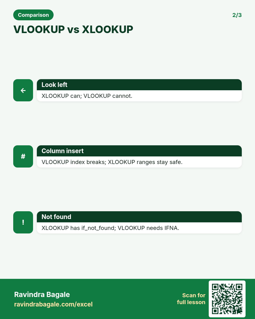
What (short answer): XLOOKUP finds a value and returns a matching result from another range. It can look left, defaults to exact match, has an if_not_found argument, and does not break when you insert columns in the middle the way VLOOKUP column index does.
How — tiny example (vertical steps):
- Ids in A, Names in B, Dept in C.
- =XLOOKUP(102,A:A,C:C,"Missing") returns Dept.
- Search can be any column — not only the first.
Formula: =XLOOKUP(102,A:A,C:C,"Missing")
Result: Finance
What it means: Department for employee 102.
INDEX + MATCH — when do you still use it?
Why interviewers ask: To see if you understand the idea, not only the button clicks.
What (short answer): INDEX returns a cell from a range by position. MATCH finds the position of a value. Together they look up in any direction and work in older Excel where XLOOKUP is missing.
How — tiny example (vertical steps):
- =MATCH("Pune",A2:A100,0) → row position.
- =INDEX(C2:C100, that_position) → result.
- Combine: =INDEX(C2:C100,MATCH("Pune",A2:A100,0)).
Formula: =INDEX(C2:C100,MATCH("Pune",A2:A100,0))
Result: West
What it means: Region for city Pune.
What does FILTER do? Give a business example.
Why interviewers ask: To see if you understand the idea, not only the button clicks.
What (short answer): FILTER spills all rows that meet conditions. Example: all overdue invoices for one salesperson. Needs Microsoft 365 or Excel 2021+.
How — tiny example (vertical steps):
- Table of invoices.
- =FILTER(A2:F500,(E2:E500<TODAY())*(D2:D500="Riya"),"None").
- Spilled block shows Riya's overdue rows.
Formula: =FILTER(A2:F500,(E2:E500<TODAY())*(D2:D500="Riya"),"None")
Result: spill of rows
What it means: Live overdue list for Riya.
UNIQUE, SORT and SORTBY — what problem do they solve?
Why interviewers ask: To see if you understand the idea, not only the button clicks.
What (short answer): UNIQUE lists distinct values. SORT sorts a range. SORTBY sorts one range by another. Together they build clean drop-downs and top-N lists without helper columns.
How — tiny example (vertical steps):
- =UNIQUE(CityColumn) for a city list.
- =SORT(that_list) for A–Z.
- =SORTBY(Products, Sales, -1) for top products.
Formula: =SORT(UNIQUE(B2:B500))
Result: sorted city list
What it means: Source for a data-validation drop-down.
How do you design a PivotTable for monthly sales by region?
Why interviewers ask: To see if you understand the idea, not only the button clicks.
What (short answer): Put Region on Rows, Month (or Date grouped by Month) on Columns, Sales on Values as Sum. Add slicers for Product. Always refresh after new data. Prefer an Excel Table as the source.
How — tiny example (vertical steps):
- Insert PivotTable from Table Sales.
- Rows: Region. Columns: Month. Values: Sum of Amount.
- Insert Slicer on Category.
Formula: Pivot: Region × Month
Result: matrix of sums
What it means: Board-ready monthly regional view.
Pivot shows Count but you need Sum — what went wrong?
Why interviewers ask: To see if you understand the idea, not only the button clicks.
What (short answer): Usually the Amount column has text numbers or blanks that made Excel choose Count. Convert to real numbers, refresh, and set Value Field Settings → Sum. Or there are mixed errors in the column.
How — tiny example (vertical steps):
- Check =ISTEXT on Amount samples.
- Fix with VALUE / Power Query type.
- Value Field Settings → Sum. Refresh.
Formula: Value Field Settings → Sum
Result: ₹ totals
What it means: Pivot now adds money, not rows.
What is Power Query used for in analyst work?
Why interviewers ask: To see if you understand the idea, not only the button clicks.
What (short answer): Power Query (Get Data / Transform) imports, cleans and reshapes data: remove columns, filter, split, unpivot, merge, append, set types. Steps refresh. Better than manual cleaning for repeat files.
How — tiny example (vertical steps):
- Data → Get Data → From Folder/CSV.
- Set types, remove duplicates, unpivot months.
- Close & Load to a Table.
Formula: (Power Query steps)
Result: clean Table
What it means: Same clean every Monday on refresh.
Merge vs Append in Power Query?
Why interviewers ask: To see if you understand the idea, not only the button clicks.
What (short answer): Append stacks tables one under another (same columns, more rows — Jan+Feb). Merge joins tables side by side like XLOOKUP (Orders + Customers on CustomerID).
How — tiny example (vertical steps):
- Append monthly files from a folder.
- Merge Orders with Customers on ID → Left Outer.
- Expand the needed customer columns.
Formula: Home → Append / Merge
Result: taller or wider table
What it means: One model instead of many copy-pastes.
Explain IFERROR and IFNA in lookup formulas.
Why interviewers ask: To see if you understand the idea, not only the button clicks.
What (short answer): IFERROR catches any error. IFNA catches only #N/A. Prefer IFNA around lookups so real errors like #REF! still show. Example: =IFNA(XLOOKUP(...),"Not found").
How — tiny example (vertical steps):
- Wrap XLOOKUP with IFNA.
- Test a missing id → Not found.
- Test a broken range → you still see #REF!.
Formula: =IFNA(XLOOKUP(A2,Ids,Names),"Not found")
Result: Not found
What it means: Missing keys handled cleanly.
How do you calculate contribution % of each product to total sales?
Why interviewers ask: To see if you understand the idea, not only the button clicks.
What (short answer): Divide each product sales by total sales. Lock the total with $ or use a Table total. Format as %. =B2/$B$10 or =B2/SUM(B:B).
How — tiny example (vertical steps):
- Product sales in B2:B9.
- In C2: =B2/SUM($B$2:$B$9).
- Fill down. Format %.
Formula: =B2/SUM($B$2:$B$9)
Result: 18%
What it means: Product share of portfolio.
What is SUMPRODUCT and when is it useful?
Why interviewers ask: To see if you understand the idea, not only the button clicks.
What (short answer): SUMPRODUCT multiplies arrays and adds the results. Useful for weighted averages and conditional sums that work in older Excel without SUMIFS arrays.
How — tiny example (vertical steps):
- Qty in B, Price in C.
- =SUMPRODUCT(B2:B10,C2:C10) → total value.
- Conditional: =SUMPRODUCT((City="Pune")*(Amount)).
Formula: =SUMPRODUCT(B2:B10,C2:C10)
Result: ₹2,45,000
What it means: Qty × Price without helper column.
You get a CSV with dates like 03/04/2026. How do you stop day/month swaps?
Why interviewers ask: To see if you understand the idea, not only the button clicks.
What (short answer): Know the source locale. In Power Query set locale when changing type to Date. In Excel use Text to Columns → Date (DMY/MDY) or DATEVALUE with care. Never trust auto-detect alone for mixed India/US files.
How — tiny example (vertical steps):
- Power Query → type Date → Using Locale → English (India) for DMY.
- Spot-check 03/04/2026 → 3 April, not 4 March.
- Add a Year-Month column after.
Formula: Change Type with Locale
Result: 3 Apr 2026
What it means: Correct month in India DMY data.
How do you find duplicates in a key column?
Why interviewers ask: To see if you understand the idea, not only the button clicks.
What (short answer): Conditional Formatting → Highlight Duplicates; or COUNTIF>1 helper; or Power Query Group By count; or Remove Duplicates on a working copy after you decide which row to keep.
How — tiny example (vertical steps):
- Helper: =COUNTIF($A$2:$A$500,A2).
- Filter helper > 1.
- Inspect before deleting.
Formula: =COUNTIF($A$2:$A$500,A2)
Result: 2+
What it means: Rows that share a repeated key.
TEXT, TEXTBEFORE, TEXTAFTER — give one cleaning example.
Why interviewers ask: To see if you understand the idea, not only the button clicks.
What (short answer): TEXT formats numbers/dates as text. TEXTBEFORE/TEXTAFTER split on a delimiter. Example: split 'SKU-7781' into prefix and number without messy MID.
How — tiny example (vertical steps):
- A2=SKU-7781.
- =TEXTBEFORE(A2,"-") → SKU.
- =TEXTAFTER(A2,"-") → 7781.
Formula: =TEXTBEFORE(A2,"-")
Result: SKU
What it means: Prefix for category grouping.
What charts do you choose for trend vs mix vs comparison?
Why interviewers ask: To see if you understand the idea, not only the button clicks.
What (short answer): Trend over time → line. Mix/share → stacked bar or pie (pie only for few parts). Compare categories → clustered column/bar. Relationship → scatter. Always label axes and avoid 3D.
How — tiny example (vertical steps):
- Monthly sales → line chart.
- Category share → bar or pie with 4–5 slices max.
- Region compare → column chart.
Formula: (chart choice)
Result: clear visual
What it means: Audience reads the message in seconds.
Manager says totals on the dashboard do not match the Pivot. How do you debug?
Why interviewers ask: To see if you understand the idea, not only the button clicks.
What (short answer): Check filters/slicers, hidden rows, Pivot cache not refreshed, Table not including new rows, calculated field vs raw sum, currency rounding, and whether cancelled orders were excluded in one place only.
How — tiny example (vertical steps):
- Refresh Pivot. Confirm source range/Table.
- Compare SUM of source vs Pivot grand total.
- Check every slicer and Report Filter.
- Document the definition of 'sales' (delivered only?).
Formula: =SUM(Table1[Amount])
Result: matches Pivot
What it means: Single definition of the KPI.
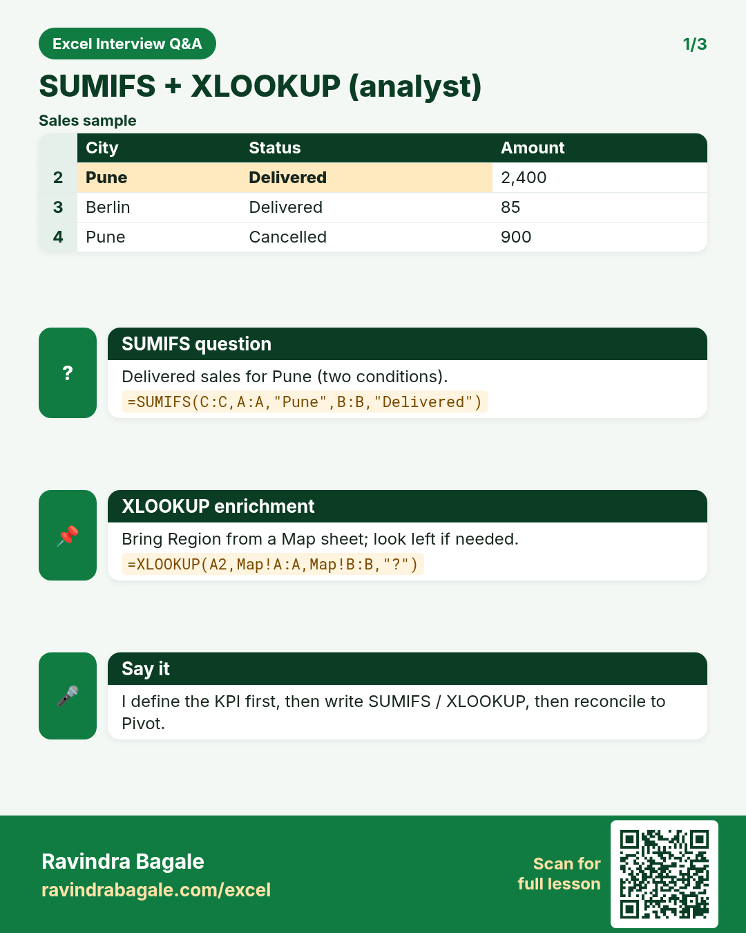
On sheet Sales, build city-wise delivered sales with SUMIFS.
Why interviewers ask: To see if you understand the idea, not only the button clicks.
What (short answer): For each city key, SUMIFS Amount where City matches and Status is Delivered. Or one Pivot with City + Status filter.
How — tiny example (vertical steps):
- Open practice file sheet Sales.
- City keys on sheet Summary.
- Write SUMIFS per city. Compare Answers.
Formula: =SUMIFS(Amount,City,A2,Status,"Delivered")
Result: see Answers
What it means: Delivered sales by city.
Create an XLOOKUP that returns Region for a City from sheet Map.
Why interviewers ask: To see if you understand the idea, not only the button clicks.
What (short answer): XLOOKUP city in Map[City] and return Map[Region]. Use if_not_found for unknown cities.
How — tiny example (vertical steps):
- On Sales add column Region.
- =XLOOKUP([@City],Map[City],Map[Region],"Check city").
- Fill via Table.
Formula: =XLOOKUP(B2,Map!A:A,Map!B:B,"Check city")
Result: West
What it means: Region enriched for Pivot.
How do you compute MoM growth %?
Why interviewers ask: To see if you understand the idea, not only the button clicks.
What (short answer): (ThisMonth - LastMonth) / LastMonth. Watch divide by zero with IF. Format as %. Example: =(B3-B2)/B2.
How — tiny example (vertical steps):
- Months in rows, sales in B.
- In C3: =IF(B2=0,NA(),(B3-B2)/B2).
- Format %.
Formula: =(B3-B2)/B2
Result: 12%
What it means: Month-over-month growth.
What is a KPI? Name five retail KPIs you can build in Excel.
Why interviewers ask: To see if you understand the idea, not only the button clicks.
What (short answer): A KPI is a number that shows progress toward a goal. Retail examples: Sales ₹, Orders, AOV (sales/orders), Return %, Gross Margin %, On-time Delivery %, Sell-through.
How — tiny example (vertical steps):
- Define formula and filters in writing.
- Build measure with SUMIFS/Pivot.
- Show vs target with variance.
Formula: =Sales/Orders
Result: AOV
What it means: Average order value.
AVERAGEIFS and median — when is average misleading?
Why interviewers ask: To see if you understand the idea, not only the button clicks.
What (short answer): AVERAGEIFS averages rows that meet conditions. Outliers pull the average. For skewed pay or order values, also show median (MEDIAN or Pivot median in newer Excel) and a trimmed view.
How — tiny example (vertical steps):
- =AVERAGEIFS(Amount,City,"Pune",Status,"Delivered").
- Also =MEDIAN on the filtered spill or helper.
- Tell the story with both.
Formula: =AVERAGEIFS(D:D,B:B,"Pune",E:E,"Delivered")
Result: ₹820
What it means: Typical delivered ticket in Pune.
How do you protect an analyst workbook before sharing?
Why interviewers ask: To see if you understand the idea, not only the button clicks.
What (short answer): Protect sheet (allow select + auto-filter), lock formula cells, leave input cells unlocked, protect workbook structure, mark file Read-only recommended. Still keep a master copy — sheet protection is not strong security.
How — tiny example (vertical steps):
- Unlock input cells (Format Cells → Protection).
- Protect Sheet with a password you store safely.
- Share PDF for one-way reading when needed.
Formula: Review → Protect Sheet
Result: formulas locked
What it means: Stakeholders edit inputs only.
You must combine 12 monthly CSVs every month. What is your plan?
Why interviewers ask: To see if you understand the idea, not only the button clicks.
What (short answer): Put them in one folder with consistent names/columns. Power Query → From Folder → Combine. Fix types once. Close & Load to Data Model or Table. Next month drop the new file and Refresh.
How — tiny example (vertical steps):
- Standardise headers in the export template.
- Build From Folder query once.
- Refresh after adding April.csv.
Formula: Get Data → From Folder
Result: all months stacked
What it means: Minutes instead of copy-paste.
Explain dynamic arrays and #SPILL!.
Why interviewers ask: To see if you understand the idea, not only the button clicks.
What (short answer): Dynamic array formulas return more than one cell. #SPILL! means something is blocking the spill range. Clear the blocking cells or move the formula.
How — tiny example (vertical steps):
- Type =UNIQUE(A2:A50) in C2.
- If D3 has old text, #SPILL! appears.
- Delete blockers or use spill refs like C2#.
Formula: =UNIQUE(A2:A50)
Result: spill list
What it means: Auto-sized distinct list.
On sheet Returns, calculate return rate % by city.
Why interviewers ask: To see if you understand the idea, not only the button clicks.
What (short answer): Return rate = Returned Amount / Gross Sales (or returned orders / orders). Align definitions. Use SUMIFS for returns and sales per city, then divide.
How — tiny example (vertical steps):
- Sales and Returns sheets share City.
- Per city: returned / sold.
- Format %. Flag cities above 5%.
Formula: =Returns/Sales
Result: 3.2%
What it means: City return rate for ops review.
What is the Data Model / Power Pivot at a high level?
Why interviewers ask: To see if you understand the idea, not only the button clicks.
What (short answer): The Data Model lets you load multiple tables and create relationships (Orders to Customers) and DAX measures. Use it when VLOOKUP merges become heavy or you need distinct counts across tables.
How — tiny example (vertical steps):
- Add tables to Data Model.
- Relate on key columns.
- Build measures like Total Sales := SUM(Sales[Amount]).
Formula: Total Sales := SUM(Sales[Amount])
Result: model measure
What it means: One measure reused in many Pivots.
Interview case: 'Sales dropped 8% MoM — how do you investigate in Excel?'
Why interviewers ask: To see if you understand the idea, not only the button clicks.
What (short answer): Break down by region, category, channel, new vs repeat. Check working days, price changes, stock-outs, big one-off clients, data issues (missing week). Use Pivot + slicers + waterfall style variance table.
How — tiny example (vertical steps):
- Pivot MoM by Region and Category.
- Find which slice explains most of the −8%.
- Validate data completeness for the month.
- Write 3 bullet insights + 1 next check.
Formula: Pivot variance view
Result: Category X −12%
What it means: Drop concentrated in one slice.
How do you create a running total in Excel?
Why interviewers ask: To see if you understand the idea, not only the button clicks.
What (short answer): In a Table: =SUM(INDEX([Amount],1):[@Amount]) or a simple expanding =SUM($B$2:B2) copied down. In a Pivot, use Running Total In on the month field. In 365, SCAN can also build it.
How — tiny example (vertical steps):
- Sort by date.
- In C2: =SUM($B$2:B2).
- Fill down. Check last row equals grand total.
Formula: =SUM($B$2:B2)
Result: cumulative ₹
What it means: Year-to-date style running total.
How do you document an analyst workbook so the next person survives?
Why interviewers ask: To see if you understand the idea, not only the button clicks.
What (short answer): Add an About sheet: source, refresh steps, KPI definitions, owner, last refresh date. Name tables and key cells. Avoid magic numbers in formulas — put rates in cells. Keep a change log.
How — tiny example (vertical steps):
- Create sheet About.
- List sources and KPI formulas in plain English.
- Colour inputs gold, outputs blue (optional legend).
Formula: (About sheet)
Result: handover ready
What it means: Anyone can refresh without a call.
XLOOKUP vs VLOOKUP vs INDEX-MATCH — 30-second comparison?
Why interviewers ask: To see if you understand the idea, not only the button clicks.
What (short answer): VLOOKUP: classic, right-only, column index fragile. INDEX-MATCH: any direction, older Excel friendly. XLOOKUP: modern default — exact match, if_not_found, left lookup, optional last match. Choose XLOOKUP when available; INDEX-MATCH for compatibility.
How — tiny example (vertical steps):
- State availability in your company Excel version.
- Pick one standard for the team.
- Show one example of left lookup.
Formula: XLOOKUP preferred
Result: team standard
What it means: Fewer silent wrong column indexes.
Practice tasks (12)
- 1. Delivered sales by city (SUMIFS) (Easy)Hint: Two conditions: city key and a status word. Sum the amount column only.
- 2. Count cancelled orders for App channel (Easy)Hint: COUNTIFS with channel and status. Exact spelling matters.
- 3. XLOOKUP region from Map sheet (Easy)Hint: Lookup city, return region, supply a not-found message.
- 4. AOV = sales / orders for each city (Medium)Hint: Divide two conditional totals. Guard against divide by zero.
- 5. MoM growth for each month row (Medium)Hint: This minus previous, divided by previous. Format as percent.
- 6. Unique sorted product list (Medium)Hint: Combine a distinct-list function with a sort function.
- 7. FILTER overdue rows for one rep (Medium)Hint: Spill rows where due date is past and owner matches.
- 8. Return rate % by city (Hard)Hint: Align units: returns over sales for the same city keys.
- 9. Pivot: Region × Month with Sum Amount (Hard)Hint: Use a Table source. Fix Values if Excel chose Count.
- 10. Running total of daily sales (Hard)Hint: Expanding range that starts at the first amount cell.
- 11. Flag duplicate Order IDs (Medium)Hint: A counting function that compares each id to the whole column.
- 12. Contribution % per product (Medium)Hint: Part divided by locked whole. Absolute reference is the key.
Quiz (8 questions)
1. SUMIFS puts which argument first?
2. XLOOKUP can look to the left?
3. Append in Power Query means:
4. #SPILL! usually means:
5. Best default for ID lookups:
6. AOV typically means:
7. Dates 03/04/2026 need care because:
8. IFNA is safer than IFERROR around lookups when:
Interview, comparison and revision cards
Standalone cards (no tip or photo strip). Each has a QR to this lesson. Download the PNG and revise offline.
Next: back to the Interview Prep hub · related lesson Formulas and Functions.