Excel Interview Prep — Fresher Basics
Friends, today we practise Excel interview questions for freshers: cells, SUM, IF, VLOOKUP, Pivot and dirty-data traps. Short answers, tiny examples, then you try on the practice file.
चला मित्रांनो — आज fresher साठी Excel interview questions: cells, SUM, IF, VLOOKUP, Pivot आणि dirty-data. छोटी उत्तरं, छोटी उदाहरणं, मग practice file.
चलो दोस्तों — आज fresher के लिए Excel interview questions: cells, SUM, IF, VLOOKUP, Pivot और dirty-data. छोटे जवाब, छोटे उदाहरण, फिर practice file.
Why → What → How
Why: Excel interviews are not memory tests of every function name. They check if you can clean a small sheet, write a correct formula, and explain the result in plain English.
What: This page has 30 real interview-style questions for Fresher Basics. Each one has a short answer, vertical steps, a tiny example, a common wrong answer, and a follow-up question.
How — study plan:
- Skim all question titles once (10 minutes).
- Download the practice workbook and open sheet
About this data. - Answer aloud, then type the formula in the file.
- Check the yellow cells on sheet
Answersonly after you try. - Revise with the three cards and take the quiz.
Download practice file: practice-fresher-interview.xlsx (includes About this data, practice sheets, Answers).
Ravindra Bagale's Tip
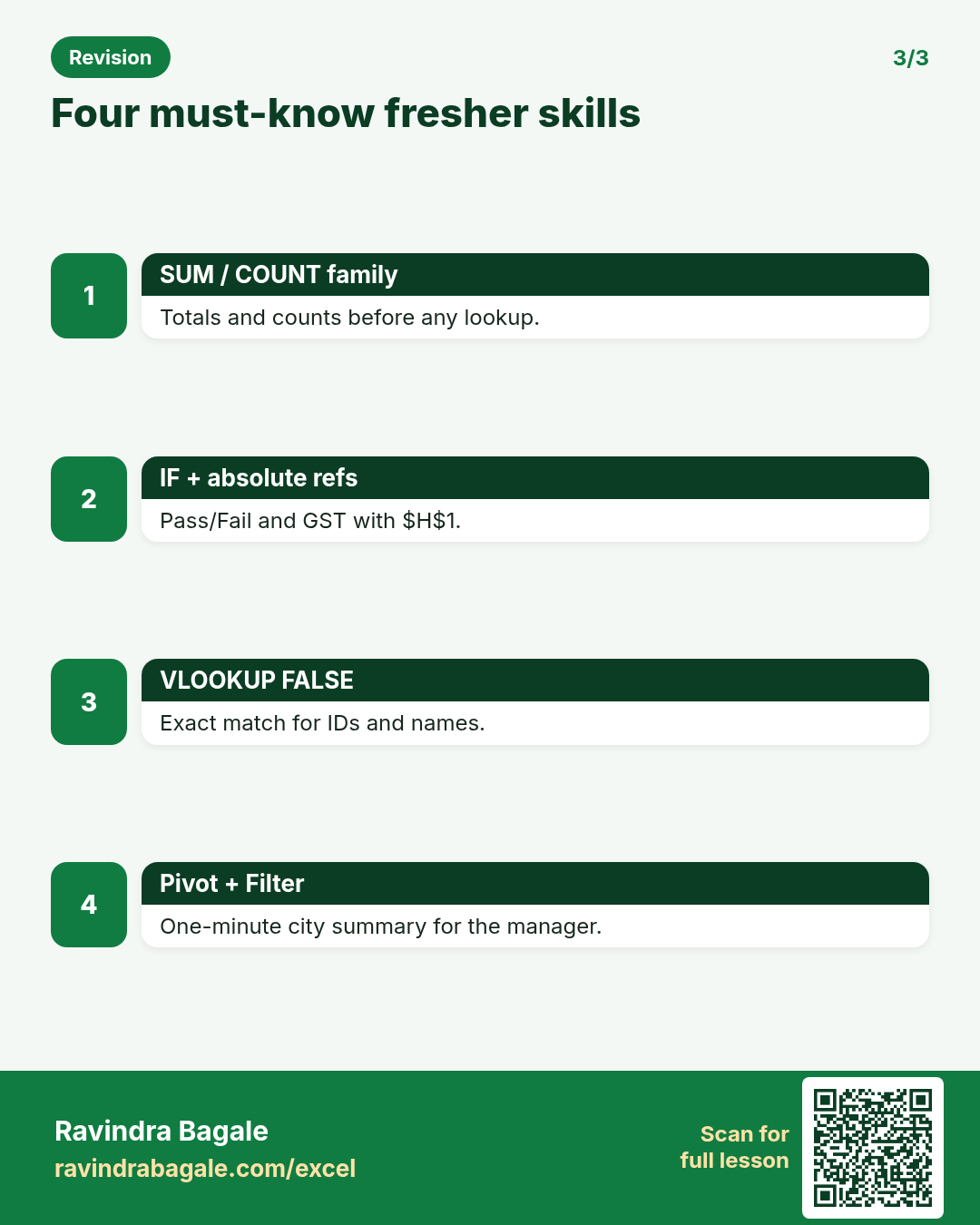
Friends, in every fresher interview they ask SUM, IF, VLOOKUP and Pivot. Practise these four until you can type them without looking.
Ravindra Bagale's Tip – मराठी
मित्रांनो, fresher interview मध्ये SUM, IF, VLOOKUP आणि Pivot विचारतात. ही चारं इतकी practise करा की न बघता type करता येतील.
Ravindra Bagale's Tip – हिंदी
दोस्तों, fresher interview में SUM, IF, VLOOKUP और Pivot पूछते हैं. ये चारों इतने practise करो कि बिना देखे type हो जाएँ.
Ravindra Bagale's Tip
Always say FALSE (exact) with VLOOKUP for IDs and names. Forgetting it is the most common fresher mistake.
Ravindra Bagale's Tip – मराठी
IDs आणि names साठी VLOOKUP मध्ये नेहमी FALSE (exact) सांगा. विसरणे ही सर्वात सामान्य fresher चूक आहे.
Ravindra Bagale's Tip – हिंदी
IDs और names के लिए VLOOKUP में हमेशा FALSE (exact) बोलो. भूलना सबसे आम fresher गलती है.
Questions (30)
What is a cell, a range and a worksheet in Excel?
Why interviewers ask: To see if you understand the idea, not only the button clicks.
What (short answer): A cell is one box (like A1). A range is a group of cells (A1:A10). A worksheet is one tab (sheet) inside a workbook.
How — tiny example (vertical steps):
- Open Excel and look at the grid.
- Click A1 — that one box is a cell.
- Drag from A1 to A5 — that is a range.
- Look at the tab at the bottom — that is a worksheet.
Formula: A1
Result: one cell
What it means: The address of a single box on the sheet.
What is the difference between a workbook and a worksheet?
Why interviewers ask: To see if you understand the idea, not only the button clicks.
What (short answer): A workbook is the whole Excel file (.xlsx). A worksheet is one sheet (tab) inside that file. One workbook can have many worksheets.
How — tiny example (vertical steps):
- Save a new file as ShopSales.xlsx — that file is the workbook.
- Add sheets named Jan, Feb, Mar — each tab is a worksheet.
- Close and reopen the file — all sheets travel together in one workbook.
Formula: (file) ShopSales.xlsx
Result: 3 sheets
What it means: One file holds many related tabs.
What does the SUM function do? Give an example.
Why interviewers ask: To see if you understand the idea, not only the button clicks.
What (short answer): SUM adds numbers in a range. Blank cells are ignored. Text that looks like numbers may cause problems — keep amounts as real numbers.
How — tiny example (vertical steps):
- Type amounts in B2:B5: 120, 80, 45, 200.
- In B6 type =SUM(B2:B5).
- Press Enter — you get 445.
Formula: =SUM(B2:B5)
Result: 445
What it means: Total of four daily sales in ₹.
Explain AVERAGE, MIN and MAX with one small example.
Why interviewers ask: To see if you understand the idea, not only the button clicks.
What (short answer): AVERAGE finds the mean. MIN finds the smallest. MAX finds the largest. All ignore blank cells.
How — tiny example (vertical steps):
- Marks in C2:C5: 72, 88, 65, 91.
- Average: =AVERAGE(C2:C5) → 79.
- Min: =MIN(C2:C5) → 65. Max: =MAX(C2:C5) → 91.
Formula: =AVERAGE(C2:C5)
Result: 79
What it means: Class average marks for four students.
What is COUNT vs COUNTA vs COUNTBLANK?
Why interviewers ask: To see if you understand the idea, not only the button clicks.
What (short answer): COUNT counts only numbers. COUNTA counts non-empty cells (text or numbers). COUNTBLANK counts empty cells.
How — tiny example (vertical steps):
- A2:A6 has: 10, apple, (blank), 20, banana.
- =COUNT(A2:A6) → 2. =COUNTA(A2:A6) → 4. =COUNTBLANK(A2:A6) → 1.
Formula: =COUNTA(A2:A6)
Result: 4
What it means: Four filled cells out of five.
Write an IF formula that shows Pass if marks are 35 or more, else Fail.
Why interviewers ask: To see if you understand the idea, not only the button clicks.
What (short answer): IF checks a condition. If true, it returns one value; if false, another. Syntax: =IF(test, value_if_true, value_if_false).
How — tiny example (vertical steps):
- Marks in D2 = 42.
- In E2 type =IF(D2>=35,"Pass","Fail").
- Result is Pass. Change D2 to 30 — result becomes Fail.
Formula: =IF(D2>=35,"Pass","Fail")
Result: Pass
What it means: Student cleared the 35-mark cut-off.
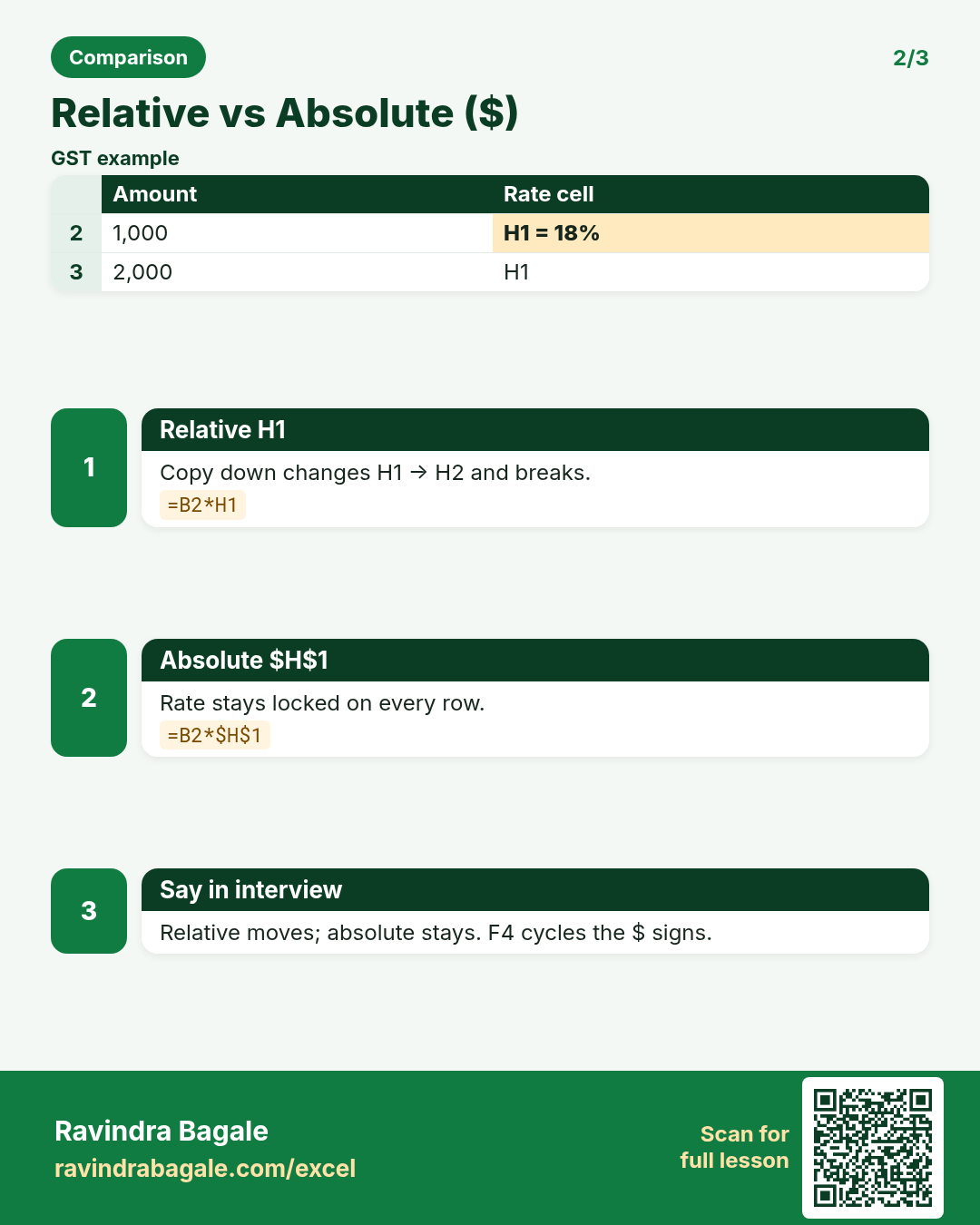
What is a relative reference vs an absolute reference ($)?
Why interviewers ask: To see if you understand the idea, not only the button clicks.
What (short answer): Relative (A1) changes when you copy the formula. Absolute ($A$1) stays fixed. Press F4 to cycle. Mixed ($A1 or A$1) locks one part.
How — tiny example (vertical steps):
- GST rate 18% is in H1. Amount in B2.
- Wrong: =B2*H1 copied down changes H1 to H2.
- Right: =B2*$H$1 — rate stays locked.
Formula: =B2*$H$1
Result: ₹1,180 if B2=1000
What it means: Amount plus GST using a fixed rate cell.
How do you join first name and last name into one cell?
Why interviewers ask: To see if you understand the idea, not only the button clicks.
What (short answer): Use & or CONCAT or TEXTJOIN. & is the simplest for two pieces. TEXTJOIN can add a space and skip blanks.
How — tiny example (vertical steps):
- A2=Priya, B2=Sharma.
- In C2 type =A2&" "&B2.
- Result: Priya Sharma.
Formula: =A2&" "&B2
Result: Priya Sharma
What it means: Full name for a letterhead.
What does TRIM do? Why do interviewers ask this?
Why interviewers ask: To see if you understand the idea, not only the button clicks.
What (short answer): TRIM removes extra spaces before, after and between words (leaves one space between words). Dirty data often has hidden spaces that break VLOOKUP.
How — tiny example (vertical steps):
- A2 has ' Pune ' with spaces.
- =TRIM(A2) → Pune.
- Now VLOOKUP can match the clean city name.
Formula: =TRIM(A2)
Result: Pune
What it means: City name ready for a clean lookup.
Explain LEFT, RIGHT and MID with one example each.
Why interviewers ask: To see if you understand the idea, not only the button clicks.
What (short answer): LEFT takes characters from the start. RIGHT from the end. MID from the middle (start position + length).
How — tiny example (vertical steps):
- Code in A2 = BLK-1001.
- =LEFT(A2,3) → BLK. =RIGHT(A2,4) → 1001. =MID(A2,5,4) → 1001.
Formula: =LEFT(A2,3)
Result: BLK
What it means: Platform code from an order id.
What is TODAY() and how is it different from a typed date?
Why interviewers ask: To see if you understand the idea, not only the button clicks.
What (short answer): TODAY() always shows today's date and updates every day. A typed date stays fixed. Use TODAY for age, overdue and 'days left' formulas.
How — tiny example (vertical steps):
- In A1 type =TODAY().
- Due date in B2 = 15-Nov-2026.
- Days left: =B2-A1.
Formula: =TODAY()
Result: current date
What it means: Live date for overdue checks.
What is Freeze Panes and why do we use it?
Why interviewers ask: To see if you understand the idea, not only the button clicks.
What (short answer): Freeze Panes keeps header rows or columns visible while you scroll. Useful for long lists so you always see column names.
How — tiny example (vertical steps):
- Select cell B2 (below header, right of first column).
- Go to View → Freeze Panes → Freeze Panes.
- Scroll down — row 1 stays. Scroll right — column A stays.
Formula: (View → Freeze Panes)
Result: headers locked
What it means: You can read 500 rows and still see titles.
What is Filter? How is it different from Sort?
Why interviewers ask: To see if you understand the idea, not only the button clicks.
What (short answer): Filter hides rows that do not match your choice (city = Pune). Sort reorders all rows (A to Z or high to low). Filter does not change order permanently; Sort does.
How — tiny example (vertical steps):
- Select the table. Data → Filter (or Ctrl+Shift+L).
- Open City drop-down → tick only Pune.
- To sort Amount high to low: Data → Sort.
Formula: Ctrl+Shift+L
Result: filter arrows on headers
What it means: Quick city-wise view without deleting rows.
What is an Excel Table (Ctrl+T) and why is it better than a plain range?
Why interviewers ask: To see if you understand the idea, not only the button clicks.
What (short answer): Ctrl+T turns a range into a Table. Benefits: auto-expand, structured names like Sales[Amount], Total Row, slicers, and formulas that copy down alone.
How — tiny example (vertical steps):
- Select A1:D20 with headers.
- Press Ctrl+T → OK.
- Add a new row under the table — it joins automatically.
Formula: =SUM(Sales[Amount])
Result: total of Amount column
What it means: Formula keeps working when rows are added.
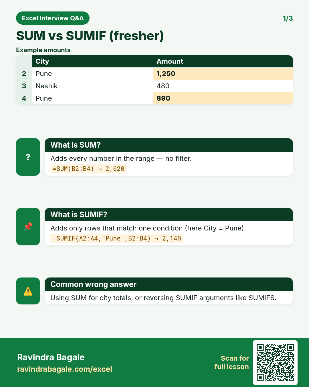
Write a SUMIF that totals sales for Mumbai only.
Why interviewers ask: To see if you understand the idea, not only the button clicks.
What (short answer): SUMIF adds values that meet one condition. Syntax: =SUMIF(range, criteria, sum_range).
How — tiny example (vertical steps):
- Cities in A2:A10. Amounts in B2:B10.
- In D2 type =SUMIF(A2:A10,"Mumbai",B2:B10).
- Only Mumbai rows are added.
Formula: =SUMIF(A2:A10,"Mumbai",B2:B10)
Result: ₹48,500
What it means: Mumbai branch sales for the week.
What does VLOOKUP do? What does the FALSE / TRUE mean?
Why interviewers ask: To see if you understand the idea, not only the button clicks.
What (short answer): VLOOKUP looks for a value in the first column of a range and returns a value from a column to its right. FALSE (or 0) = exact match. TRUE = approximate match (needs sorted data).
How — tiny example (vertical steps):
- Ids in A2:A5, Names in B2:B5.
- =VLOOKUP(102,A2:B5,2,FALSE) returns the name for id 102.
- Always use FALSE for IDs and names.
Formula: =VLOOKUP(102,A2:B5,2,FALSE)
Result: Ananya
What it means: Employee name for code 102.
Your VLOOKUP returns #N/A. What do you check first?
Why interviewers ask: To see if you understand the idea, not only the button clicks.
What (short answer): Check: (1) exact spelling and spaces (TRIM), (2) number stored as text vs real number, (3) lookup value really missing, (4) column index too big, (5) table range cut off.
How — tiny example (vertical steps):
- Compare lookup cell and table cell with =A2=D2.
- Wrap both sides with TRIM and VALUE if needed.
- Use IFERROR to show a friendly message after you fix data.
Formula: =IFERROR(VLOOKUP(A2,T,2,FALSE),"Not found")
Result: Not found
What it means: Clean message instead of #N/A on screen.
What is Conditional Formatting? Give one interview example.
Why interviewers ask: To see if you understand the idea, not only the button clicks.
What (short answer): Conditional Formatting changes a cell's colour or icon based on a rule — for example, mark sales below target in red.
How — tiny example (vertical steps):
- Select Amount column.
- Home → Conditional Formatting → Highlight Cells → Less Than → 5000.
- Low sales turn red automatically.
Formula: rule: cell < 5000
Result: red fill
What it means: Manager sees weak days at a glance.
What is Data Validation? Why use a drop-down list?
Why interviewers ask: To see if you understand the idea, not only the button clicks.
What (short answer): Data Validation limits what users can type. A drop-down list forces City to be only from an allowed list — fewer spelling mistakes.
How — tiny example (vertical steps):
- Select City column.
- Data → Data Validation → List → Source: Pune,Mumbai,Nashik.
- Users pick from the list; wrong spellings are blocked.
Formula: List: Pune,Mumbai,Nashik
Result: drop-down in cell
What it means: Clean city names for SUMIF and Pivot.
On the practice sheet Orders, find total Amount for Status = Delivered.
Why interviewers ask: To see if you understand the idea, not only the button clicks.
What (short answer): Use SUMIF on Status and Amount. Or filter Delivered and read the Total Row of a Table.
How — tiny example (vertical steps):
- Open sheet Orders.
- In a blank cell type =SUMIF(StatusRange,"Delivered",AmountRange).
- Match your answer with the check cell on sheet Answers (yellow).
Formula: =SUMIF(E:E,"Delivered",D:D)
Result: see Answers!B2
What it means: Only delivered sales counted.
Create a Pass/Fail column for marks using IF.
Why interviewers ask: To see if you understand the idea, not only the button clicks.
What (short answer): Add a helper column. If Marks >= 35 show Pass, else Fail. Copy the formula down or use a Table so it auto-fills.
How — tiny example (vertical steps):
- On sheet Marks, column C has marks.
- In D2: =IF(C2>=35,"Pass","Fail").
- Fill down. Count passes with COUNTIF.
Formula: =IF(C2>=35,"Pass","Fail")
Result: Pass or Fail
What it means: Ready for a count of pass students.
What does ROUND do? ROUND vs INT?
Why interviewers ask: To see if you understand the idea, not only the button clicks.
What (short answer): ROUND(number, digits) rounds to that many decimals. INT strips decimals toward zero for positive numbers (floors). ROUND(2.5,0)=3; INT(2.9)=2.
How — tiny example (vertical steps):
- Price 199.567 in A2.
- =ROUND(A2,2) → 199.57 for money.
- =INT(A2) → 199.
Formula: =ROUND(A2,2)
Result: 199.57
What it means: Money shown with two paise digits.
Boss asks: 'How many unique cities are in this list?' What do you do as a fresher?
Why interviewers ask: To see if you understand the idea, not only the button clicks.
What (short answer): Easy ways: select the city column → Data → Remove Duplicates on a copy; or use UNIQUE function (=UNIQUE(A2:A100)) in Microsoft 365; or PivotTable with City in Rows.
How — tiny example (vertical steps):
- Copy City column to a new sheet.
- Data → Remove Duplicates.
- COUNTA the remaining list. Or =COUNTA(UNIQUE(A2:A100)).
Formula: =COUNTA(UNIQUE(A2:A100))
Result: 7
What it means: Seven different cities in the file.
Name five useful Excel shortcuts and what they do.
Why interviewers ask: To see if you understand the idea, not only the button clicks.
What (short answer): Ctrl+C copy, Ctrl+V paste, Ctrl+Z undo, Ctrl+S save, Ctrl+Arrow jump to edge, Ctrl+Shift+L filter, F4 absolute ref, Alt+= AutoSum, Ctrl+T table, Ctrl+; today's date.
How — tiny example (vertical steps):
- Practice Alt+= on a number column.
- Practice Ctrl+Shift+L on a table.
- Practice F4 inside a formula.
Formula: Alt+=
Result: =SUM(...)
What it means: AutoSum writes SUM for you.
What file types do you know: xlsx, csv, xls?
Why interviewers ask: To see if you understand the idea, not only the button clicks.
What (short answer): xlsx is the modern Excel workbook. csv is plain text with commas (no formulas or formatting). xls is the old Excel 97–2003 format. Prefer xlsx for work; use csv to share raw data.
How — tiny example (vertical steps):
- Save As → Excel Workbook (*.xlsx).
- Save As → CSV UTF-8 for data exchange.
- Never email an important dashboard only as csv.
Formula: Save As *.xlsx
Result: formulas kept
What it means: Workbook stays fully editable.
Explain COUNTIF with an example.
Why interviewers ask: To see if you understand the idea, not only the button clicks.
What (short answer): COUNTIF counts cells that match one condition. =COUNTIF(range, criteria).
How — tiny example (vertical steps):
- Status in E2:E20.
- =COUNTIF(E2:E20,"Cancelled") counts cancelled orders.
- Use "Pune" on a city column for city count.
Formula: =COUNTIF(E2:E20,"Cancelled")
Result: 3
What it means: Three cancelled orders this week.
A colleague pasted numbers that will not sum. What could be wrong?
Why interviewers ask: To see if you understand the idea, not only the button clicks.
What (short answer): Numbers stored as text (green corner), leading spaces, currency symbols typed as text, or hidden characters from PDF/web paste. Fix with VALUE, Paste Special → Multiply by 1, Text to Columns, or NUMBERVALUE.
How — tiny example (vertical steps):
- =ISTEXT(A2) to test.
- Type 1 in a cell, copy, Paste Special → Multiply on the column.
- Or =VALUE(TRIM(A2)).
Formula: =VALUE(TRIM(A2))
Result: 1250
What it means: Text '1,250' becomes a real number.
What is a PivotTable in one sentence? When would a fresher use it?
Why interviewers ask: To see if you understand the idea, not only the button clicks.
What (short answer): A PivotTable summarises many rows into a compact table (sum/count by city, month, product) without writing formulas. Freshers use it for sales by city or headcount by department.
How — tiny example (vertical steps):
- Select the data → Insert → PivotTable.
- Drag City to Rows, Amount to Values.
- Change Values to Sum or Count as needed.
Formula: Insert → PivotTable
Result: City-wise sales
What it means: One-minute summary for the manager.
On sheet Staff, find how many employees are in HR using COUNTIF.
Why interviewers ask: To see if you understand the idea, not only the button clicks.
What (short answer): Point COUNTIF at the Department column with criteria "HR".
How — tiny example (vertical steps):
- Open sheet Staff.
- Department is column C.
- =COUNTIF(C:C,"HR") or a tight range C2:C50.
- Check Answers!B3.
Formula: =COUNTIF(C2:C50,"HR")
Result: see Answers!B3
What it means: Headcount in HR for the interview task.
How should you answer 'Tell me about yourself' in an Excel fresher interview?
Why interviewers ask: To see if you understand the idea, not only the button clicks.
What (short answer): Keep it short: your course or degree, that you practised Excel formulas and PivotTables on sample data (say Blinkit-style or college marks), one concrete example you built, and that you want to learn more on the job. Do not list every function.
How — tiny example (vertical steps):
- Prepare a 45-second version.
- Name one file you built (attendance, marks, sales).
- Offer to open Excel and show if asked.
Formula: (spoken answer)
Result: clear 45-sec intro
What it means: Confidence + one proof of skill.
Practice tasks (12)
- 1. Total of all order amounts (Easy)Hint: Use one function that adds a whole column of numbers. Ignore the header.
- 2. Count how many orders exist (Easy)Hint: Count non-blank Order IDs — not the amount column.
- 3. Total sales for Pune only (Easy)Hint: One condition: city name. Add the matching amounts.
- 4. How many Delivered orders? (Easy)Hint: Count rows where Status matches one word exactly.
- 5. Pass or Fail from marks (Medium)Hint: Write a logical test against 35. Return two text labels.
- 6. Full name from first + last (Medium)Hint: Join two cells with a space in the middle. Avoid the plus sign.
- 7. Clean city names with spaces (Medium)Hint: Remove leading and trailing spaces without deleting the city word.
- 8. GST amount at 18% locked rate (Medium)Hint: Amount times rate. Lock the rate cell so copy-down stays correct.
- 9. Pune + Delivered total (Hard)Hint: Two conditions at once. Think of the function that allows many criteria.
- 10. Unique city count (Hard)Hint: Either UNIQUE+COUNTA, or a Pivot, or Remove Duplicates on a copy.
- 11. Highlight amounts under ₹5,000 (Medium)Hint: Use a rule that paints cells — do not colour by hand.
- 12. Drop-down for Status (Medium)Hint: Restrict the cell to a short list of allowed words.
Quiz (8 questions)
1. COUNT counts which cells?
2. To lock cell H1 in a formula you write:
3. Best exact-match VLOOKUP flag:
4. Ctrl+T creates a:
5. TRIM mainly removes:
6. TODAY() returns:
7. SUMIF needs how many required ideas?
8. Numbers that will not SUM are often:
Interview, comparison and revision cards
Standalone cards (no tip or photo strip). Each has a QR to this lesson. Download the PNG and revise offline.
Next: back to the Interview Prep hub · related lesson Formulas and Functions.