Excel VLOOKUP Function
Chala mitrano — today VLOOKUP. Look in the first column, count across to the answer column, and almost always use FALSE for an exact match.
चला मित्रांनो — आज VLOOKUP. पहिल्या column मध्ये शोधा, उजवीकडे column count करा, आणि नेहमी जवळजवळ FALSE (exact match) वापरा.
चलो दोस्तों — आज VLOOKUP. पहली column में खोजो, दाईं ओर column गिनो, और लगभग हमेशा FALSE (exact match) इस्तेमाल करो.
Purpose
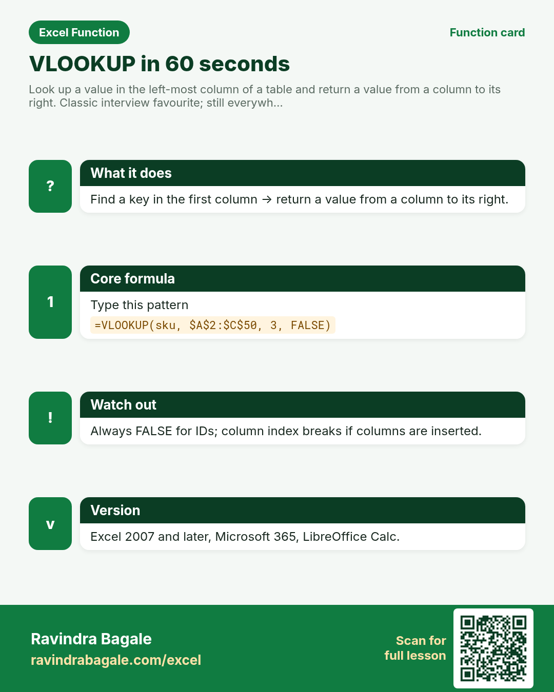
Look up a value in the left-most column of a table and return a value from a column to its right. Classic interview favourite; still everywhere in older workbooks.
Return value
The value from the chosen column of the matching row, or #N/A if nothing matches (exact mode).
Syntax
Arguments
| Argument | Required? | Description |
|---|---|---|
lookup_value | Required | The value to find in the first column of table_array (SKU, ID, name, or a cell). |
table_array | Required | The full table range. First column must hold the lookup keys; return columns sit to the right. |
col_index_num | Required | Which column to return, counting from 1 at the left of table_array (2 = second column). |
range_lookup | Optional | FALSE or 0 = exact match (use this almost always). TRUE or 1 = approximate; table must be sorted ascending. |
Version
Excel 2007 and later, Microsoft 365, LibreOffice Calc. Prefer XLOOKUP on Microsoft 365 when you can.
How to use — Why → What → How
Why: Price lists, employee codes and store IDs live in tables. You need the matching price or city without scanning by hand. In Indian back offices VLOOKUP is still the first lookup people learn. A purchase team in Nagpur keeps SKU in column A and price in column C; a UK sister store in Manchester mirror...
What: VLOOKUP finds lookup_value in the first column of table_array and returns the cell from column col_index_num of that row. Read the arguments table carefully; each one changes the answer in a specific way.
How — numbered steps:
- Click the cell where the answer should appear.
- Type =VLOOKUP( then click the lookup cell (example: SKU in F2).
- Select the whole table (first column = keys). Press F4 once to add $ locks.
- Type the column number to return (2 for the second column, 3 for the third…).
- Type FALSE for exact match, close the bracket, press Enter. Fill down if needed.
- Compare your result with the Answers sheet only after you attempt it.
- Write one sentence in your own words explaining when you would use this function at work.
Ravindra Bagale's Tip
Friends, lock the table with $ (example $A$2:$D$50) before you fill down. Without $, the table slides and answers go wrong.
Ravindra Bagale's Tip – मराठी
मित्रांनो, fill down करण्यापूर्वी table ला $ लावा ($A$2:$D$50). $ नसेल तर table सरकते आणि उत्तरे चुकीची येतात.
Ravindra Bagale's Tip – हिंदी
दोस्तों, fill down से पहले table को $ से लॉक करो ($A$2:$D$50). $ न हो तो table सरकती है और जवाब गलत आते हैं.
Ravindra Bagale's Tip
Column index is a number, not a header name. If someone inserts a column, the number can silently point to the wrong field — that is why XLOOKUP is safer.
Ravindra Bagale's Tip – मराठी
Column index ही संख्या आहे, header नाव नाही. Column insert झाले तर चुकीचे field येऊ शकते — म्हणून XLOOKUP सुरक्षित आहे.
Ravindra Bagale's Tip – हिंदी
Column index एक संख्या है, header नाम नहीं. Column insert हो तो गलत field आ सकता है — इसलिए XLOOKUP सुरक्षित है.
Ravindra Bagale's Tip
Friends, after class open a blank sheet and rebuild one VLOOKUP example without looking. That memory test beats re-reading the page.
Ravindra Bagale's Tip – मराठी
मित्रांनो, class नंतर रिकाम्या sheet वर VLOOKUP चे एक उदाहरण न पाहता पुन्हा लिहा. हे memory test पृष्ठ पुन्हा वाचण्यापेक्षा जास्त मदत करते.
Ravindra Bagale's Tip – हिंदी
दोस्तों, class के बाद खाली sheet पर VLOOKUP का एक उदाहरण बिना देखे फिर से लिखो. यह memory test पेज दोबारा पढ़ने से ज़्यादा मदद करता है.
Download practice file: practice-vlookup.xlsx (includes sheet About this data, practice sheets, and Answers).
Worked examples
1) Exact match — price for a SKU
Nagpur warehouse sheet. Find the ₹ price for SKU-104.
| SKU | Item | Price (₹) |
|---|---|---|
| SKU-101 | Atta 5kg | 420 |
| SKU-104 | Oil 1L | 189 |
| SKU-107 | Rice 10kg | 780 |
Result: 189
What it means: Excel finds SKU-104 in column 1 and returns column 3 (Price) from the same row.
2) Exact match missing — #N/A
Someone typed SKU-999 which is not in the list.
| SKU | Item | Price (₹) |
|---|---|---|
| SKU-101 | Atta 5kg | 420 |
| SKU-104 | Oil 1L | 189 |
Result: #N/A
What it means: No exact key. Wrap with IFNA to show a friendly message in reports.
3) Return city for a store code (₹ / £ mix)
Store master: India and UK codes in one list.
| Store | City | Currency |
|---|---|---|
| ST-11 | Nagpur | ₹ |
| ST-18 | Manchester | £ |
| ST-22 | Pune | ₹ |
Result: Manchester
What it means: Lookup key ST-18; column index 2 returns City.
4) Approximate match for tax slab (sorted table)
Income slabs sorted ascending. Find the tax % for income 85,000.
| Income from | Tax % |
|---|---|
| 0 | 0% |
| 50000 | 5% |
| 80000 | 10% |
| 120000 | 15% |
Result: 10%
What it means: TRUE finds the largest key ≤ 85000, which is 80000 → 10%.
5) Friendly message with IFNA
MIS report must never show a red #N/A for a missing SKU.
| SKU | Price (₹) |
|---|---|
| SKU-101 | 420 |
| SKU-104 | 189 |
Result: Not in list
What it means: IFNA catches only #N/A and replaces it with clean text.
6) Fill-down with locked table
Many SKUs in column F; table stays in A:C.
| SKU | Price (₹) |
|---|---|
| SKU-101 | 420 |
| SKU-104 | 189 |
| SKU-107 | 780 |
Result: (price for whatever SKU is in F2)
What it means: Absolute refs keep the table fixed when you copy the formula down.
Common errors and fixes
Notes and tips
- VLOOKUP can only return columns to the right of the key column. For left-side returns use INDEX+MATCH or XLOOKUP.
- Default range_lookup is TRUE — dangerous for IDs. Type FALSE every time unless you truly need a sorted approximate match.
- Duplicate keys: VLOOKUP returns the first match only.
- On Microsoft 365, teach XLOOKUP first; still learn VLOOKUP because older files and interviews use it.
- In Indian back offices VLOOKUP is still the first lookup people learn. A purchase team in Nagpur keeps SKU in column A and price in column C; a UK sister store in Manchester mirrors the same layout with pound prices. Exact match with FALSE (or 0) is the safe habit for codes. Approximate match with TRUE is only for sorted numeric slabs such as tax or discount bands. When a colleague inserts a column between Item and Price, every col_index_num silently shifts — that single pain point is why modern teams move to XLOOKUP or INDEX plus MATCH. Practice locking the table with dollar signs before you fill down, and wrap reports with IFNA so missing SKUs show clear text instead of red #N/A.
- VLOOKUP vs XLOOKUP: VLOOKUP needs the key on the left and a column number; XLOOKUP takes separate lookup and return arrays, can search either side, and has a built-in if_not_found. Learn both: VLOOKUP for legacy and interviews, XLOOKUP for new Microsoft 365 work.
- Fictional sample data only — practice amounts and names are made for learning.
- After you finish the 10 tasks, re-read the errors table once; most class mistakes are listed there.
- Keep ranges locked with absolute references when you copy formulas down a column of inputs.
- Say the business question in plain words before you type the equals sign — it prevents wrong arguments.
In real work
In Indian back offices VLOOKUP is still the first lookup people learn. A purchase team in Nagpur keeps SKU in column A and price in column C; a UK sister store in Manchester mirrors the same layout with pound prices. Exact match with FALSE (or 0) is the safe habit for codes. Approximate match with TRUE is only for sorted numeric slabs such as tax or discount bands. When a colleague inserts a column between Item and Price, every col_index_num silently shifts — that single pain point is why modern teams move to XLOOKUP or INDEX plus MATCH. Practice locking the table with dollar signs before you fill down, and wrap reports with IFNA so missing SKUs show clear text instead of red #N/A.
How it compares
VLOOKUP vs XLOOKUP: VLOOKUP needs the key on the left and a column number; XLOOKUP takes separate lookup and return arrays, can search either side, and has a built-in if_not_found. Learn both: VLOOKUP for legacy and interviews, XLOOKUP for new Microsoft 365 work.
Interview corner
- Why do interviewers still ask VLOOKUP if XLOOKUP exists?
- Because millions of legacy files and shared templates still use it, and it proves you understand exact vs approximate match.
- What breaks when someone inserts a column?
- The numeric col_index_num no longer points at the same field, so answers look plausible but wrong.
- How do you look left with VLOOKUP?
- You cannot. Reshape the table, or use INDEX+MATCH / XLOOKUP.
Related functions
XLOOKUP, INDEX, MATCH, HLOOKUP, IFNA
Practice tasks (10)
- Task 1. On sheet Stock, return Price for SKU-104 in cell G2 (exact match).Hint: column index for Price — count from the left of the table.
- Task 2. In G3, look up SKU-999 and show Not in list when missing.Hint: wrap VLOOKUP with IFNA.
- Task 3. Return City for store ST-18.Hint: City is column 2 of the store table.
- Task 4. Write a fill-down formula that looks up the SKU in F2 with a locked table.Hint: press F4 on the table range.
- Task 5. Explain in one line why inserting a column can break VLOOKUP silently.Hint: think about the column index number.
- Task 6. Using approximate match, find the tax % for income 85,000 on the Tax sheet.Hint: range_lookup TRUE; table must stay sorted.
- Task 7. Change your Price lookup so a blank SKU cell shows Enter SKU.Hint: IF or IFNA around VLOOKUP.
- Task 8. Return the Item name (not price) for SKU-107.Hint: different column index.
- Task 9. Find what happens if you omit FALSE on an unsorted ID list — write the wrong result you see.Hint: compare with and without FALSE.
- Task 10. Bonus: return Currency symbol for ST-11.Hint: third column of the store table.
Quick quiz
Answers: Q1=False, Q2=FALSE, Q3=The left of table_array, Q4=#N/A, Q5=IFNA or IFERROR (check after you try).
Revision card
Standalone card (no tip or photo strip). QR opens this lesson. Download the PNG and revise offline.