Excel SUMIFS Function
Chala mitrano — today SUMIFS. One sum, many filters. City, status, date — stack the conditions and Excel adds only the matching rows.
चला मित्रांनो — आज SUMIFS. एक sum, अनेक filters. City, status, date — conditions स्टॅक करा; Excel फक्त जुळणाऱ्या rows जोडेल.
चलो दोस्तों — आज SUMIFS. एक sum, कई filters. City, status, date — शर्तें जोड़ो; Excel सिर्फ matching rows जोड़ेगा.
Purpose
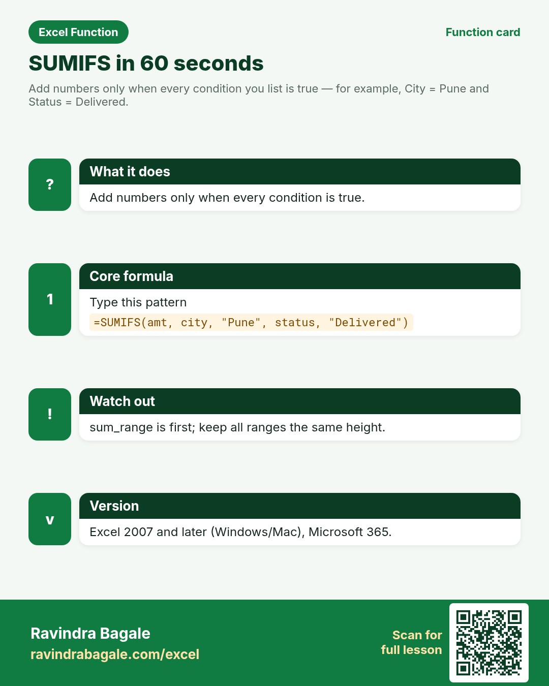
Add numbers only when every condition you list is true — for example, City = Pune and Status = Delivered.
Return value
A single number: the sum of sum_range cells that pass all criteria. Returns 0 when nothing matches.
Syntax
Arguments
| Argument | Required? | Description |
|---|---|---|
sum_range | Required | The cells to add (must be numbers). |
criteria_range1 | Required | The first range to test. |
criteria1 | Required | The test for that range (number, text, cell, or expression like ">100"). |
criteria_range2, criteria2, … | Optional | More range/criteria pairs. All pairs must pass for a row to be included. |
Version
Excel 2007 and later (Windows/Mac), Microsoft 365. Supported in LibreOffice Calc.
How to use — Why → What → How
Why: A plain SUM adds everything. Business questions need “only Delivered in Pune” or “only VIP in March”.
What: SUMIFS walks row by row: if all criteria pass, that row’s sum_range value is added.
How — numbered steps:
- Decide which column to add (Amount).
- Type =SUMIFS( and select the Amount column first.
- Select the first filter column (City), comma, then the criterion ("Pune" or a cell).
- Add more pairs for Status, Date, etc.
- Close the bracket and press Enter. Check the total against a filtered view once.
Ravindra Bagale's Tip
Friends, put sum_range first — opposite of SUMIF’s order. Mixing the order is the number-one SUMIFS typo in class.
Ravindra Bagale's Tip – मराठी
मित्रांनो, sum_range पहिला — SUMIF च्या उलट. Order बदलणे ही class मधील सर्वात सामान्य चूक आहे.
Ravindra Bagale's Tip – हिंदी
दोस्तों, sum_range पहले आता है — SUMIF से उलटा. Order बदलना class की सबसे आम गलती है.
Ravindra Bagale's Tip
Keep every criteria_range the same shape as sum_range (same number of rows). Uneven ranges give wrong totals or errors.
Ravindra Bagale's Tip – मराठी
प्रत्येक criteria_range ची shape sum_range सारखी ठेवा. असमान ranges चुकीची totals देतात.
Ravindra Bagale's Tip – हिंदी
हर criteria_range की shape sum_range जैसी रखो. असमान ranges गलत totals देती हैं.
Download practice file: practice-sumifs.xlsx (includes sheet About this data, practice sheets, and Answers).
Worked examples
1) One city total
Add Amount where City is Pune.
| City | Amount (₹) |
|---|---|
| Pune | 400 |
| Dubai | 150 |
| Pune | 250 |
Result: 650
What it means: Only the two Pune rows are added: 400 + 250.
2) City + status
Pune and Delivered only.
| City | Status | Amount |
|---|---|---|
| Pune | Delivered | 400 |
| Pune | Cancelled | 200 |
| Dubai | Delivered | 150 |
Result: 400
What it means: Cancelled Pune is skipped; Dubai is skipped.
3) Numeric criterion
Sum amounts greater than 200.
| Order | Amount |
|---|---|
| A1 | 180 |
| A2 | 220 |
| A3 | 310 |
Result: 530
What it means: 220 + 310. The criteria range can be the same as sum_range.
4) Cell reference as criterion
City name sits in E1 so the manager can change it.
| City | Amount |
|---|---|
| Pune | 400 |
| Dubai | 150 |
| Pune | 250 |
Result: 650
What it means: Changing E1 to Dubai recalculates without editing the formula.
5) Wildcards for partial text
Sum all channels that start with App.
| Channel | Amount |
|---|---|
| App-iOS | 90 |
| App-Android | 110 |
| Web | 70 |
Result: 200
What it means: * means any characters after App.
6) Mixed currency sheet — sum AED rows only
Dubai cafe rows stored as AED amounts.
| City | Currency | Amount |
|---|---|---|
| Pune | INR | 400 |
| Dubai | AED | 120 |
| Dubai | AED | 80 |
Result: 200
What it means: Only AED rows; do not mix INR and AED in one KPI without converting.
Common errors and fixes
Notes and tips
- SUMIFS is AND logic across criteria. For OR, use several SUMIFS added together, or FILTER in Microsoft 365.
- Text criteria are not case-sensitive in Excel.
- Empty criterion cells can accidentally match blanks — prefer a real input cell with data validation.
Related functions
SUMIF, COUNTIFS, AVERAGEIFS, SUM, FILTER
Practice tasks (10)
- Task 1. Sum Amount for City = Pune on sheet Sales.Hint: sum_range first, then City range and "Pune".
- Task 2. Sum Amount for Pune and Status = Delivered.Hint: two criteria pairs.
- Task 3. Sum Amount where Amount > 200.Hint: criteria can point at the Amount column itself.
- Task 4. Put a city name in H1 and sum using H1 as the criterion.Hint: no quotes around H1.
- Task 5. Sum all Channel values that start with App.Hint: wildcard *.
- Task 6. Sum only AED currency rows.Hint: filter on the Currency column.
- Task 7. Sum Delivered orders for Dubai.Hint: City and Status together.
- Task 8. Compare your Pune total with a manual filter — do they match?Hint: Data → Filter, then read the status bar sum.
- Task 9. Write why SUMIFS(0) can still be “correct”.Hint: think about filters that exclude every row.
- Task 10. Bonus: sum Pune Delivered where Amount >= 250.Hint: three criteria pairs.
Quick quiz
Answers: Q1=sum_range, Q2=False, Q3=">100", Q4=0 (check after you try).
Revision card
Standalone card (no tip or photo strip). QR opens this lesson. Download the PNG and revise offline.