Excel XLOOKUP Function
Chala mitrano — today we learn XLOOKUP. It is the modern replacement for VLOOKUP: look left or right, and give a clear message when the ID is missing.
चला मित्रांनो — आज XLOOKUP शिकू. हे VLOOKUP चं आधुनिक रूप आहे: डावीकडे किंवा उजवीकडे शोध, आणि ID नसेल तर स्वच्छ message.
चलो दोस्तों — आज XLOOKUP सीखते हैं. यह VLOOKUP का नया रूप है: बाएँ या दाएँ दोनों तरफ खोज, और ID न मिले तो साफ़ message.
Purpose
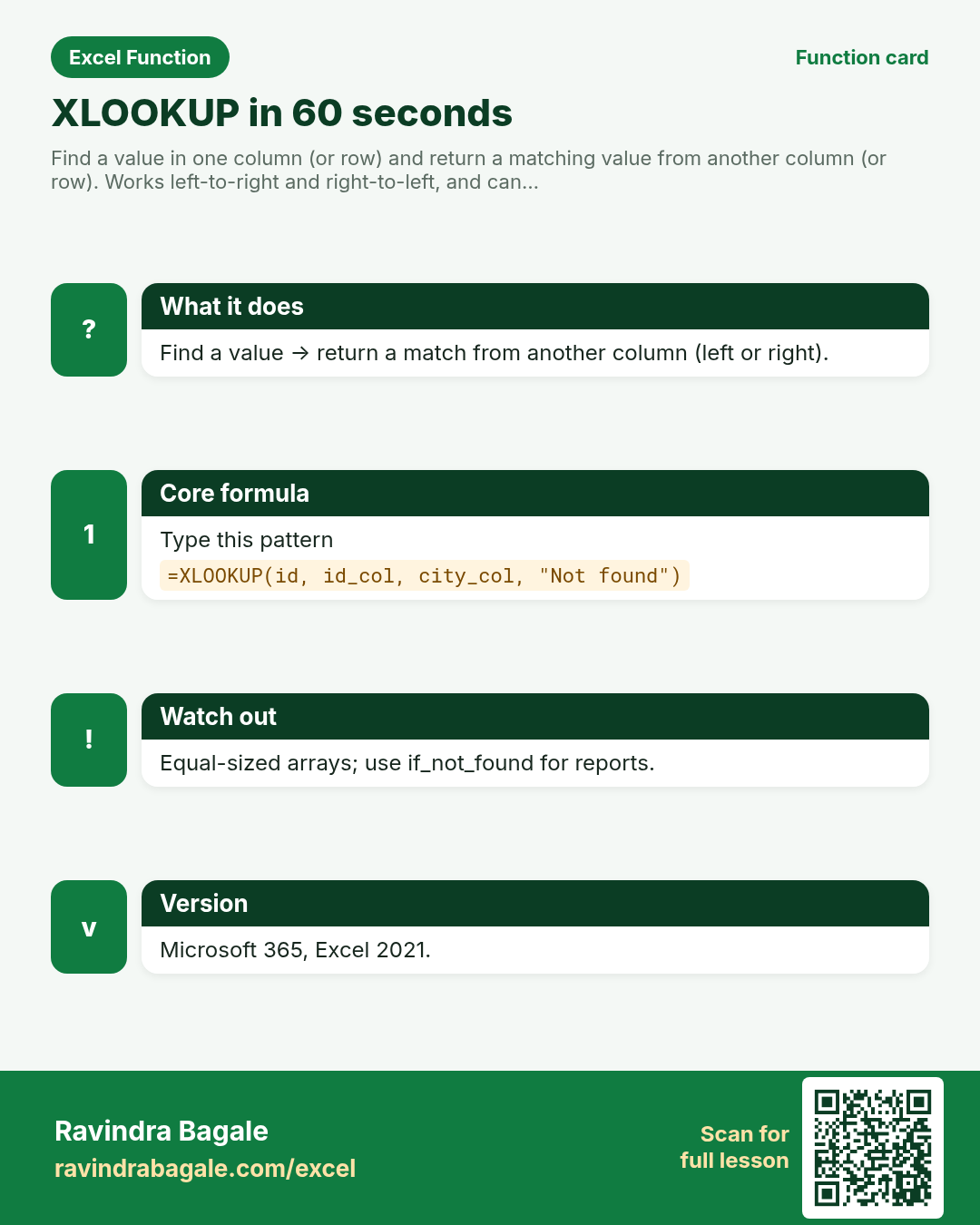
Find a value in one column (or row) and return a matching value from another column (or row). Works left-to-right and right-to-left, and can return a friendly message when nothing matches.
Return value
The matching value from the return array, or the if_not_found value you set. Can also return multiple columns when combined with other functions.
Syntax
Arguments
| Argument | Required? | Description |
|---|---|---|
lookup_value | Required | The value you want to find (cell, number, or text). |
lookup_array | Required | The one-column (or one-row) range to search in. |
return_array | Required | The one-column (or one-row) range to return from. Same height/width as lookup_array. |
if_not_found | Optional | What to show when nothing matches (text or value). If omitted, Excel shows #N/A. |
match_mode | Optional | 0 exact (default), -1 exact or next smaller, 1 exact or next larger, 2 wildcard. |
search_mode | Optional | 1 first-to-last (default), -1 last-to-first, 2 binary asc, -2 binary desc. |
Version
Microsoft 365, Excel 2021. Not in Excel 2019 or older. LibreOffice Calc: limited / may be missing — use INDEX+MATCH as a fallback there.
How to use — Why → What → How
Why: VLOOKUP can only look to the right and breaks when you insert a column. Interviews and real MIS sheets need a lookup that stays stable and can search either side.
What: XLOOKUP searches lookup_array for lookup_value and returns the matching cell from return_array. Optional arguments control “not found”, wildcards and search direction.
How — numbered steps:
- Click the cell where the answer should appear.
- Type =XLOOKUP( then click the lookup value (example: order ID).
- Select the lookup column (IDs), comma, then the return column (City or Amount).
- Add a fourth argument like "Not found" so missing IDs stay readable.
- Press Enter. Copy the formula down if you need many rows.
Ravindra Bagale's Tip
Friends, always put if_not_found for IDs and phone numbers. A clean “Not found” looks better in a report than a red #N/A.
Ravindra Bagale's Tip – मराठी
मित्रांनो, IDs आणि phone numbers साठी नेहमी if_not_found द्या. Report मध्ये स्वच्छ “Not found” हे लाल #N/A पेक्षा चांगले दिसते.
Ravindra Bagale's Tip – हिंदी
दोस्तों, IDs और phone numbers के लिए हमेशा if_not_found दो. Report में साफ़ “Not found” लाल #N/A से बेहतर लगता है.
Ravindra Bagale's Tip
Keep lookup_array and return_array the same height. If one is longer, XLOOKUP can spill wrong or throw #VALUE!.
Ravindra Bagale's Tip – मराठी
lookup_array आणि return_array ची उंची सारखी ठेवा. एक लांब असेल तर #VALUE! येऊ शकतो.
Ravindra Bagale's Tip – हिंदी
lookup_array और return_array की ऊँचाई एक जैसी रखो. एक लंबा हो तो #VALUE! आ सकता है.
Download practice file: practice-xlookup.xlsx (includes sheet About this data, practice sheets, and Answers).
Worked examples
1) Exact match — city for an order ID
Small kirana sheet. Find the city for order ORD-104.
| Order | City | Amount (₹) |
|---|---|---|
| ORD-101 | Pune | 1,250 |
| ORD-104 | Nashik | 890 |
| ORD-107 | Pune | 2,100 |
Result: Nashik
What it means: Excel finds ORD-104 in the Order column and returns the City from the same row.
2) Friendly message when ID is missing
Manager typed ORD-999 by mistake.
| Order | City |
|---|---|
| ORD-101 | Pune |
| ORD-104 | Nashik |
Result: Not found
What it means: No match, so the fourth argument appears instead of #N/A.
3) Look to the left (VLOOKUP cannot do this)
City is in column A; Order ID is in column B. Return the order for Nashik.
| City | Order |
|---|---|
| Pune | ORD-101 |
| Nashik | ORD-104 |
| Birmingham | ORD-110 |
Result: ORD-104
What it means: Lookup array is City; return array is Order — left-side return works naturally.
4) Return amount in £ for a UK order
Same list has a Birmingham order in pounds.
| Order | City | Amount |
|---|---|---|
| ORD-101 | Pune | ₹1,250 |
| ORD-110 | Birmingham | £48.50 |
| ORD-104 | Nashik | ₹890 |
Result: £48.50
What it means: Exact match on ORD-110 returns the Amount cell as stored.
5) Last match with search_mode -1
Customer Priya placed two orders; you want the latest row.
| Customer | Order |
|---|---|
| Priya Sharma | ORD-101 |
| James Cole | ORD-102 |
| Priya Sharma | ORD-118 |
Result: ORD-118
What it means: search_mode -1 starts from the bottom, so the last Priya row wins.
Common errors and fixes
Notes and tips
- Default match is exact (match_mode 0) — safer than VLOOKUP’s approximate habit.
- Wildcards (* and ?) need match_mode 2.
- For many columns back, people often nest XLOOKUP or use FILTER; keep examples simple first.
- On Excel 2019 and older, use INDEX + MATCH instead.
Related functions
VLOOKUP, INDEX, MATCH, FILTER, IFNA
Practice tasks (10)
- Task 1. On sheet Orders, return City for order ORD-104 in cell G2.Hint: lookup the Order column; return the City column.
- Task 2. In G3, look up ORD-999 and show the text Missing ID when not found.Hint: use the fourth argument.
- Task 3. In G4, return Amount for Birmingham’s order (look up by City).Hint: City can be the lookup_array.
- Task 4. Find the last order ID for customer Priya Sharma.Hint: search_mode is the sixth argument.
- Task 5. Return the Amount for ORD-110 (UK row).Hint: exact match on Order; return Amount.
- Task 6. Write an XLOOKUP that returns Not in list for a blank lookup cell.Hint: still set if_not_found; test with an empty cell.
- Task 7. Change your City lookup so a wrong spelling shows Check spelling.Hint: fourth argument is just text.
- Task 8. Using the practice file, return City for the order in cell F2 (cell reference, not typed text).Hint: lookup_value should be F2, not a quoted ID.
- Task 9. Explain in one line why XLOOKUP is safer than VLOOKUP when someone inserts a column.Hint: think about column index numbers.
- Task 10. Bonus: return Amount for ORD-101 and format the result cell as ₹.Hint: formula first; number format is separate.
Quick quiz
Answers: Q1=True, Q2=if_not_found, Q3=Last match, Q4=False (check after you try).
Revision card
Standalone card (no tip or photo strip). QR opens this lesson. Download the PNG and revise offline.