Excel → Power BI Bridge
Bridge 4. PivotTables → matrix & visuals
Friends,
Friends, your Pivot muscle still works. Rows, Columns, Values, Filters become Matrix fields and slicers. Watch currency.
चला मित्रांनो
चला मित्रांनो, तुमचा Pivot स्नायू चालतो. Rows/Columns/Values/Filters → Matrix आणि slicers. Currency लक्षात ठेवा.
चलो दोस्तों
चलो दोस्तों, आपका Pivot मांसपेशी काम करती है. Rows/Columns/Values/Filters → Matrix और slicers. Currency ध्यान रखो.
At deploy, files go to s3://ravindrabagale-cards/excel/bridge/ .
What you will learn
- Map Pivot Rows/Columns/Values/Filters to Matrix + slicers.
- Use Show Values As ideas via quick measures carefully.
- Keep currency out of a blind SUM.
- Build the same question in Excel Pivot and a Matrix plan.
A short story
Amit’s Nashik desk wants City down the side and Industry across — classic Pivot. In Desktop that shape is a Matrix, with Currency on a slicer so INR never hugs GBP.
Ravindra Bagale’s Tip
Never drop mixed currencies into one Values well without a rule. Filter or convert first.
Ravindra Bagale’s Tip – मराठी
मिश्र currencies एक Values मध्ये टाकू नका — आधी filter किंवा convert.
Ravindra Bagale’s Tip – हिंदी
मिश्र currencies एक Values में मत डालो — पहले filter या convert.
1. Field list → Matrix wells
Friends,
If the Matrix looks empty, check filters and relationships — not only the visual.
चला मित्रांनो
Matrix रिकामा असेल तर filters/relationships तपासा.
चलो दोस्तों
Matrix खाली हो तो filters/relationships जाँचो.
Why: Same mental model, new UI.
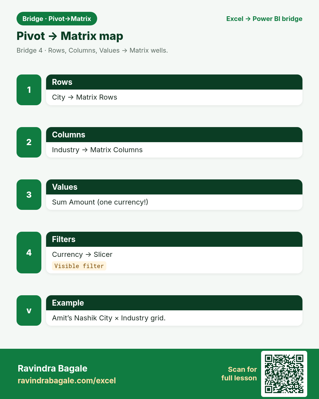
What: Rows / Columns / Values / Filters.
How:
- Create a Matrix visual.
- Drag City to Rows, Industry to Columns.
- Drag Amount to Values.
- Put Currency on a slicer, not silently in Values.
| Excel | Power BI / DAX | Result | Meaning |
|---|---|---|---|
Excel PivotRows=City, Columns=Industry |
Power BIMatrix + slicer |
Grid |
Pune Retail vs IT cells appear. |
2. Report filters become slicers
Friends,
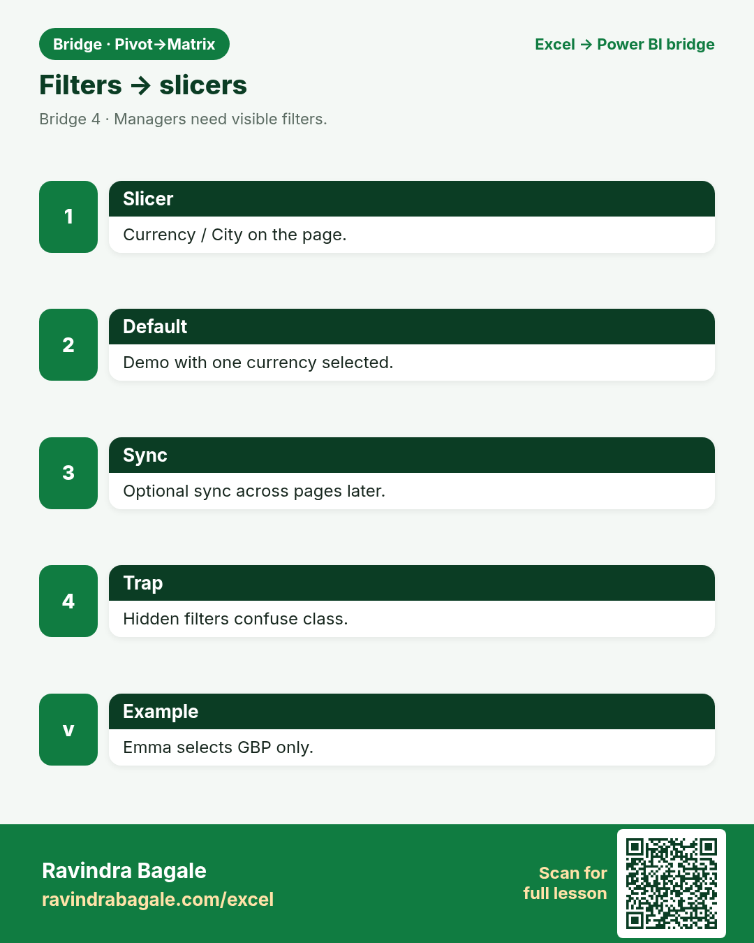
Visible filters beat hidden page-level traps in class demos.
चला मित्रांनो
दिसणारे filters चांगले — लपलेले page filters गोंधळ करतात.
चलो दोस्तों
दिखते filters बेहतर — छिपे page filters उलझाते हैं.
Why: Slicers are friendlier for managers.
What: Currency / City slicers sync across visuals.
How:
- Insert slicer for Currency.
- Optionally sync slicers across pages later.
- Keep one clear default (e.g. INR).
- Do not hide a dangerous filter with no UI.
| Excel | Power BI / DAX | Result | Meaning |
|---|---|---|---|
ExcelPivot Filter / slicer |
Power BISlicer visual |
Filtered |
Emma sees only GBP when she needs it. |
3. Values and aggregation
Friends,
Name measures Total Sales vs Order Count so nobody guesses.
चला मित्रांनो
Total Sales आणि Order Count वेगळे नाव द्या.
चलो दोस्तों
Total Sales और Order Count अलग नाम दो.
Why: Sum is not always right.
What: Count of OrderID vs Sum of Amount.
How:
- Ask: count orders or sum money?
- Use Count for OrderID; Sum for Amount.
- Watch blanks — they are not zeros.
- Separate measures later for clarity.
| Excel | Power BI / DAX | Result | Meaning |
|---|---|---|---|
ExcelSummarize by Sum/Count |
Power BIDefault Sum; change in well |
Clear |
Omar’s fee count ≠ fee sum. |
4. Show Values As → quick ideas
Friends,
DIVIDE protects you from divide-by-zero better than plain /.
चला मित्रांनो
DIVIDE zero-divide पासून वाचवते.
चलो दोस्तों
DIVIDE zero-divide से बचाता है.
Why: % of total is a habit in Pivot.
What: Quick measures / DIVIDE patterns.
How:
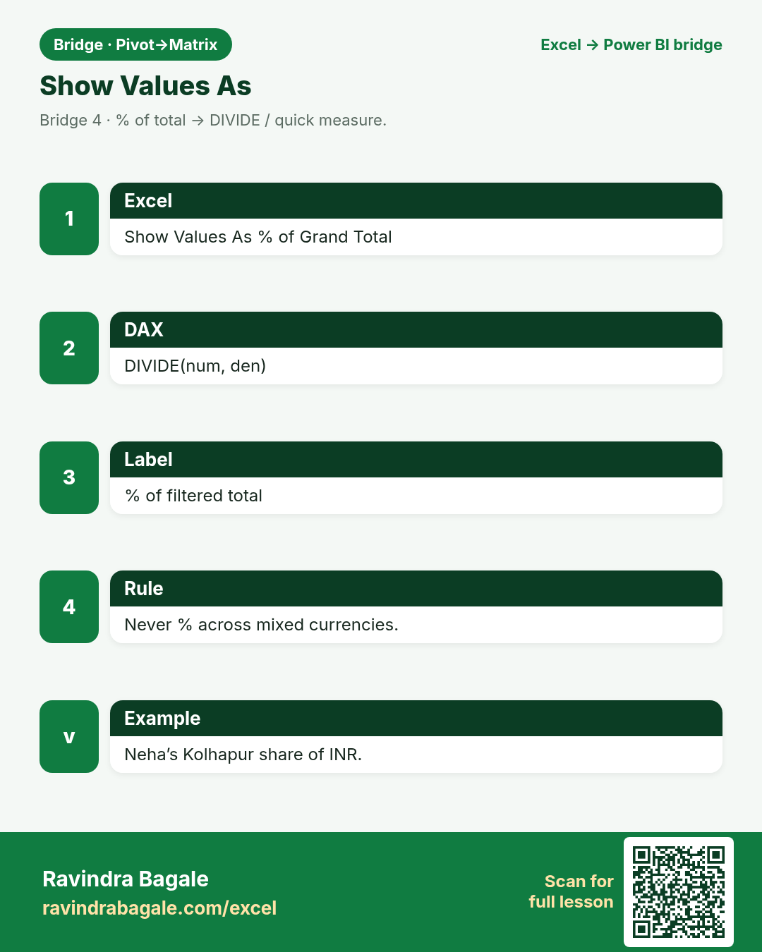
- In Pivot: Show Values As % of Grand Total.
- In PBI: quick measure or DIVIDE(num, den).
- Never % across mixed currencies.
- Label the visual “% of filtered total”.
| Excel | Power BI / DAX | Result | Meaning |
|---|---|---|---|
ExcelShow Values As |
Power BIQuick measure / DIVIDE |
% |
Neha’s Kolhapur share of INR total. |
5. Matrix design habits
Friends,
A Matrix plus one Card often beats a Matrix that tries to shout every total.
चला मित्रांनो
Matrix + एक Card अनेकदा पुरेसे.
चलो दोस्तों
Matrix + एक Card अक्सर काफ़ी.
Why: Stepped layout, subtotals, word wrap.
What: Turn off noisy totals when teaching.
How:
- Toggle row subtotals if they confuse beginners.
- Resize columns; turn on word wrap for long names.
- Use a clear title: Sales by City × Industry.
- Add a card for Grand Total beside the Matrix.
| Excel | Power BI / DAX | Result | Meaning |
|---|---|---|---|
ExcelDesign tab on Pivot |
Power BIFormat visual pane |
Readable |
Sofia’s Berlin class can read City names. |
6. Sort and top N
Friends,
Top N without a currency rule is a trap question in exams and in life.
चला मित्रांनो
Currency शिवाय Top N = सापळा.
चलो दोस्तों
Currency के बिना Top N = जाल.
Why: Managers ask for top 5 cities.
What: Sort by Amount; filter Top N carefully.
How:
- Sort Matrix by Value descending.
- Top N via filters pane / visual level.
- Say which currency the Top N uses.
- Compare with Excel Pivot Top 10 filter.
| Excel | Power BI / DAX | Result | Meaning |
|---|---|---|---|
ExcelTop 10 filter |
Power BIFilter pane Top N |
Top cities |
Priya’s Pune stays visible in INR Top N. |
7. Multiple visuals, one question
Friends,
One page, one story. Extra visuals need a reason.
चला मित्रांनो
एक page, एक गोष्ट. अतिरिक्त visuals ला कारण हवे.
चलो दोस्तों
एक page, एक कहानी. अतिरिक्त visuals की वजह चाहिए.
Why: Pivot is one grid. Desktop is a page.
What: Matrix + line + slicer answer richer questions.
How:
- Keep Matrix for comparison.
- Add a line for monthly trend (later data).
- Same slicer drives both.
- Do not build six Matrices that ask the same thing.
| Excel | Power BI / DAX | Result | Meaning |
|---|---|---|---|
ExcelOne Pivot sheet |
Power BIPage of visuals |
Story |
Ananya’s IT pack: Matrix + trend. |
8. When to stay on Excel Pivot
Friends,
The bridge respects Excel. It relocates shared truth.
चला मित्रांनो
Bridge Excel ला सन्मान देते. Shared truth हलवते.
चलो दोस्तों
Bridge Excel का सम्मान करता है. Shared truth हिलाता है.
Why: Small personal grids are fine.
What: Bridge, do not ban.
How:
- Personal scratch analysis → Excel Pivot OK.
- Shared board used by 12 managers → Matrix on a model.
- Analyze in Excel can reconnect later.
- Pick tools by audience size and refresh need.
| Excel | Power BI / DAX | Result | Meaning |
|---|---|---|---|
ExcelLocal Pivot |
Power BIPublished Matrix |
Choice |
Chen Wei drafts in Excel, publishes in PBI. |
Practice tasks (12)
Use bridge-pivot-practice.xlsx. LibreOffice-safe: prefer SUMIF / VLOOKUP / IF — avoid XLOOKUP, TEXTJOIN, TEXTSPLIT.
- Read About this data. Note the currency warning.
Hint
First sheet.
- On Pivot_Source, build an Excel Pivot: City rows, Industry columns, Sum Amount.
Hint
Classic layout.
- Add Currency as a Pivot filter; set INR only.
Hint
Avoid mixed sum.
- Fill Matrix_Plan column gaps in your own words.
Hint
Rows/Columns/Values/Filters.
- Write why Amount+mixed Currency is dangerous.
Hint
Notes sheet.
- Compute Pune total with SUMIF (LibreOffice-safe).
Hint
=SUMIF(City,"Pune",Amount)
- Count Manchester rows with COUNTIF.
Hint
Orders ≠ money.
- Propose a Top 3 cities rule that names currency.
Hint
INR Top 3…
- Sketch one page: Matrix + Currency slicer + Card.
Hint
Notes.
- List Show Values As → DIVIDE idea in one sentence.
Hint
% of filtered total.
- Flag any blank City with IF.
Hint
Data quality.
- Write when you would keep a local Excel Pivot instead.
Hint
Personal scratch.
Quick quiz
Q1. Pivot Rows map closest to…
Q2. Currency for managers should usually be a…
Q3. Sum of Amount across INR+GBP without a rule is…
Q4. Show Values As % becomes which habit in DAX?
Q5. Order Count should use…
Q6. Top N must state…
Q7. A Matrix + Card is often better than…
Q8. Personal scratch Pivot in Excel is…
Loading practice tasks...
- Rows in the fact table (Easy): How many orders are in the Sales table?
- Total amount (Easy): Add up the Amount column of Sales.
- Total quantity (Easy): Add up the Qty column of Sales.
- Products in the dimension (Easy): How many products are in the Products table?
- Products actually sold (Medium): How many of the 5 Product IDs (P01 to P05) appear at least once in Sales?
- Amount for one city (Medium): Add up Amount where City is "London".
- Product name through the relationship (Medium): What is the Product name for Product ID "P03"?
- Sales of one product (Medium): Add up Amount where Product ID is "P03".
- Average order amount (Medium): Find the average Amount, rounded to 0 decimals.
- Category of the first order (Hard): Find the Category of the product in the first order.
- Biggest order in London (Hard): What is the largest Amount where City is "London"?
- Share of P03 (Hard): What share of the total Amount comes from Product ID "P03"? Round to 3 decimals.
Quick revision cards (3)
Approved Excel card style: standalone, no tip/photo section, QR to this lesson.