Excel → Power BI Bridge
Bridge 3. Excel formulas → DAX
Friends,
Friends, today we translate Excel formulas into DAX. Same questions. New home. We keep LibreOffice-safe Excel practice in the workbook, and we show the Power BI measure next to it.
चला मित्रांनो
चला मित्रांनो, आज Excel formulas DAX मध्ये भाषांतर. तोच प्रश्न. नवीन घर. Workbook मध्ये LibreOffice-safe Excel practice, आणि बाजूला Power BI measure.
चलो दोस्तों
चलो दोस्तों, आज Excel formulas का DAX में अनुवाद. वही सवाल. नया घर. Workbook में LibreOffice-safe Excel practice, और साथ में Power BI measure.
Practice workbook and revision cards load from s3://ravindrabagale-cards/excel/bridge/.
What you will learn
- Rewrite SUMIFS / COUNTIFS thinking as CALCULATE measures.
- Replace most VLOOKUP pulls with relationships + RELATED.
- Use IF, SWITCH, and DIVIDE safely.
- Respect filter context and currency rules.
A short story
Amit keeps six SUMIFS blocks for Nashik. Ananya copies COUNTIFS for Hyderabad tickets. Every new city means another paste. One model with a few measures ends that copy-paste life — after you map the formulas honestly.
Ravindra Bagale’s Tip
Always write the base measure (plain SUM) before CALCULATE variants. Name measures like Total Amount (INR) when currency matters.
Ravindra Bagale’s Tip – मराठी
CALCULATE variant आधी base measure (साधा SUM) लिहा. Currency महत्त्वाची असेल तर Total Amount (INR) सारखी नावे द्या.
Ravindra Bagale’s Tip – हिंदी
CALCULATE variant से पहले base measure (सादा SUM) लिखो. Currency मायने रखे तो Total Amount (INR) जैसे नाम दो.
1. Formula mindset → measure mindset
Friends,
Friends, a measure is a smart calculator. Filters walk in; the number walks out.
चला मित्रांनो
चला मित्रांनो — measure म्हणजे हुशार कॅल्क्युलेटर. Filters येतात; नंबर बाहेर येतो.
चलो दोस्तों
चलो दोस्तों — measure यानी स्मार्ट कैलकुलेटर. Filters आते हैं; नंबर निकलता है.
Why: In Excel you often write a formula in a cell next to data. In Power BI you usually write a measure that reacts to filters.
What: Cell formulas vs measures in filter context.
How:
- Excel: put =SUM(C:C) or =SUMIFS(...) in a cell or table column.
- Power BI: create a measure Total Sales = SUM(Sales[Amount]).
- Drop the measure on a visual. Slicers change the answer automatically.
- Do not paste the same SUMIFS in 40 cells — one measure serves all visuals.
| Excel | Power BI / DAX | Result | Meaning |
|---|---|---|---|
Excel cell=SUMIFS(Amount,City,"Pune") |
DAX measurePune Sales = CALCULATE(SUM(Sales[Amount]), Sales[City]="Pune") |
₹1,25,000 |
Priya’s Pune kirana total when City slicer = Pune (or hard-filtered). |
2. SUMIFS → CALCULATE
Friends,
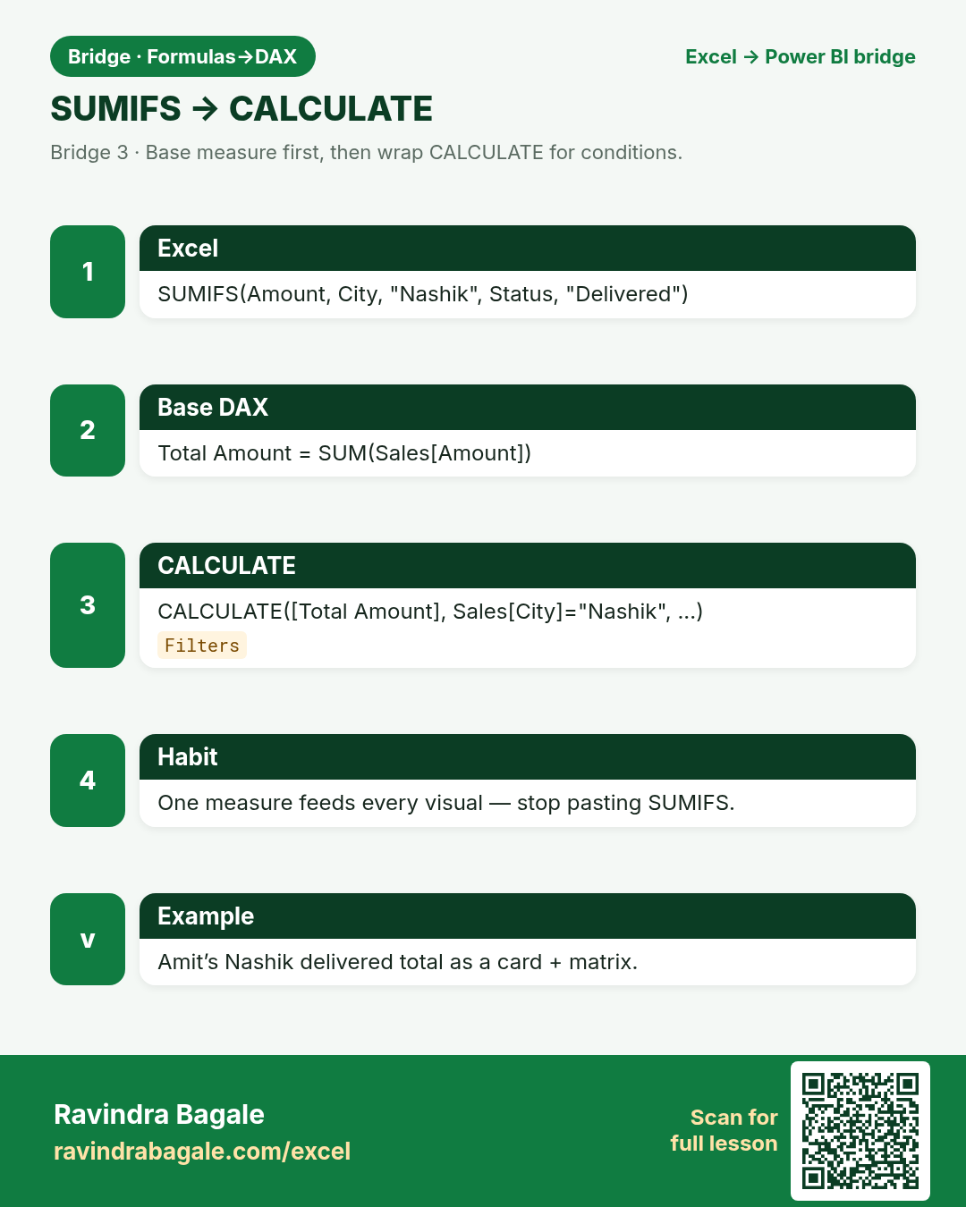
Base measure first. Then wrap CALCULATE. Copy-paste SUMIFS into 20 cards is the old world.
चला मित्रांनो
आधी base measure. मग CALCULATE. वीस cards मध्ये SUMIFS पेस्ट करणे = जुने जग.
चलो दोस्तों
पहले base measure. फिर CALCULATE. बीस cards में SUMIFS पेस्ट = पुरानी दुनिया.
Why: SUMIFS is the Excel comfort food for “total where…”. CALCULATE is the DAX door for the same idea — and more.
What: Replace multi-condition SUMIFS with CALCULATE + filters (or slicers).
How:
- Write the base measure first: Total Amount = SUM(Sales[Amount]).
- Add conditions with CALCULATE(Total Amount, Sales[City]="Nashik", Sales[Status]="Delivered").
- Prefer letting slicers filter the base measure when the report is interactive.
- Remember: CALCULATE can also remove filters (ALL) — power that SUMIFS does not give easily.
| Excel | Power BI / DAX | Result | Meaning |
|---|---|---|---|
Excel=SUMIFS(Amount,City,"Nashik",Status,"Delivered") |
DAXCALCULATE([Total Amount], Sales[City]="Nashik", Sales[Status]="Delivered") |
₹42,300 |
Amit’s Nashik branch delivered lines only. |
3. COUNTIF / COUNTIFS → COUNTROWS + FILTER / CALCULATE
Friends,
COUNTBLANK friends: use CALCULATE with BLANK checks carefully — blanks are not always zero.
चला मित्रांनो
COUNTBLANK मित्रांनो: BLANK तपासताना काळजी — रिकामे नेहमी शून्य नसते.
चलो दोस्तों
COUNTBLANK दोस्तों: BLANK जाँचते समय सावध — खाली हमेशा शून्य नहीं.
Why: Counting rows under conditions is daily work in retail and IT tickets.
What: COUNTROWS of a filtered table, or CALCULATE(COUNTROWS(...), ...).
How:
- Excel: =COUNTIFS(Status,"Open",City,"Hyderabad").
- DAX option A: CALCULATE(COUNTROWS(Tickets), Tickets[Status]="Open", Tickets[City]="Hyderabad").
- DAX option B: COUNTROWS(FILTER(Tickets, Tickets[Status]="Open" && Tickets[City]="Hyderabad")).
- Prefer CALCULATE style for measures that must respect slicers cleanly.
| Excel | Power BI / DAX | Result | Meaning |
|---|---|---|---|
Excel=COUNTIFS(Status,"Open",City,"Hyderabad") |
DAXCALCULATE(COUNTROWS(Tickets), Tickets[Status]="Open", Tickets[City]="Hyderabad") |
17 |
Ananya’s open IT tickets in Hyderabad. |
4. VLOOKUP / XLOOKUP → relationships + RELATED
Friends,
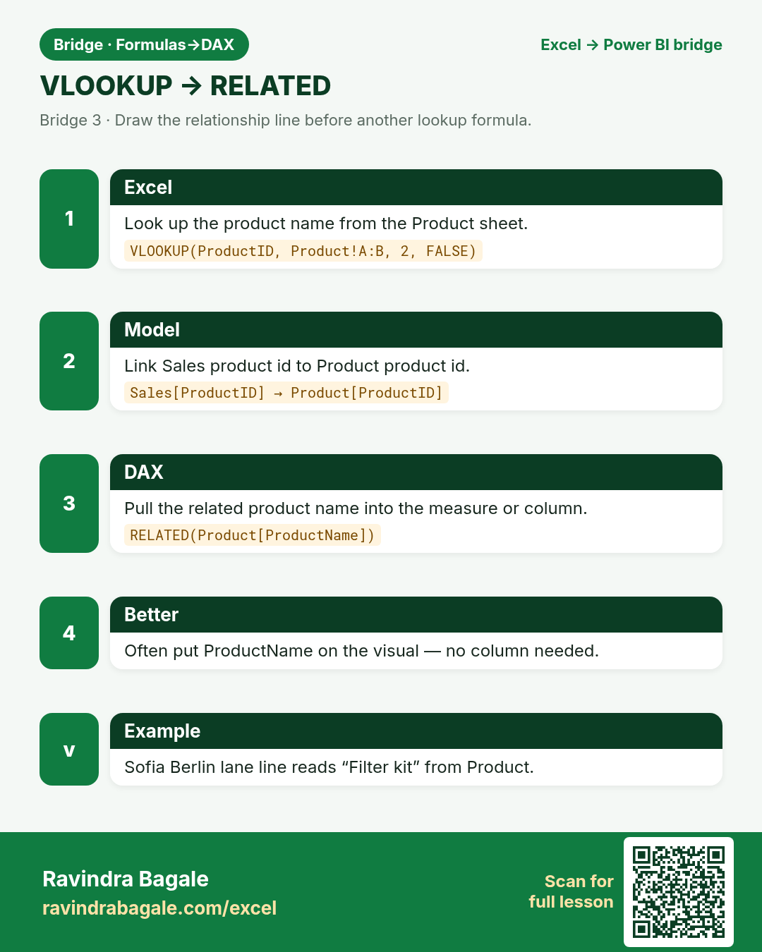
If you still VLOOKUP inside Power BI like Excel, pause. Draw the relationship line first.
चला मित्रांनो
Power BI मध्ये Excel सारखे VLOOKUP करत असाल तर थांबा. आधी relationship ओळ काढा.
चलो दोस्तों
Power BI में Excel जैसा VLOOKUP कर रहे हो तो रुकें. पहले relationship रेखा खींचो.
Why: Looking up a name from an ID is the classic second-sheet problem. Models replace most lookups.
What: Relate tables on the key; pull the column with RELATED in a calculated column, or just use the field in visuals.
How:
- Do not load a wide flat table with ProductName pasted on every fact row if you can help it.
- Load Sales and Product. Model view: Sales[ProductID] many-to-one Product[ProductID].
- In a calculated column on Sales: Product Name = RELATED(Product[ProductName]).
- Often you need no column — put Product[ProductName] on the visual axis directly.
- LOOKUPVALUE exists for odd cases; relationships are the default habit.
| Excel | Power BI / DAX | Result | Meaning |
|---|---|---|---|
Excel=VLOOKUP(A2,Product!A:B,2,FALSE) |
DAXRELATED(Product[ProductName]) (after relationship) |
Atta 5kg |
Sofia’s Berlin lane line gets the product label from Product table. |
5. IF → IF / SWITCH
Friends,
Nested IF over three levels? Try SWITCH. Your future self will thank you.
चला मित्रांनो
तीन पातळ्यांपेक्षा जास्त nested IF? SWITCH वापरा. भविष्यातील तुम्ही धन्यवाद द्याल.
चलो दोस्तों
तीन स्तर से ज़्यादा nested IF? SWITCH इस्तेमाल करो. भविष्य का तुम धन्यवाद देगा.
Why: Branching logic moves almost one-to-one, with SWITCH for clean multi-label maps.
What: IF for two-way tests; SWITCH for status → label maps.
How:
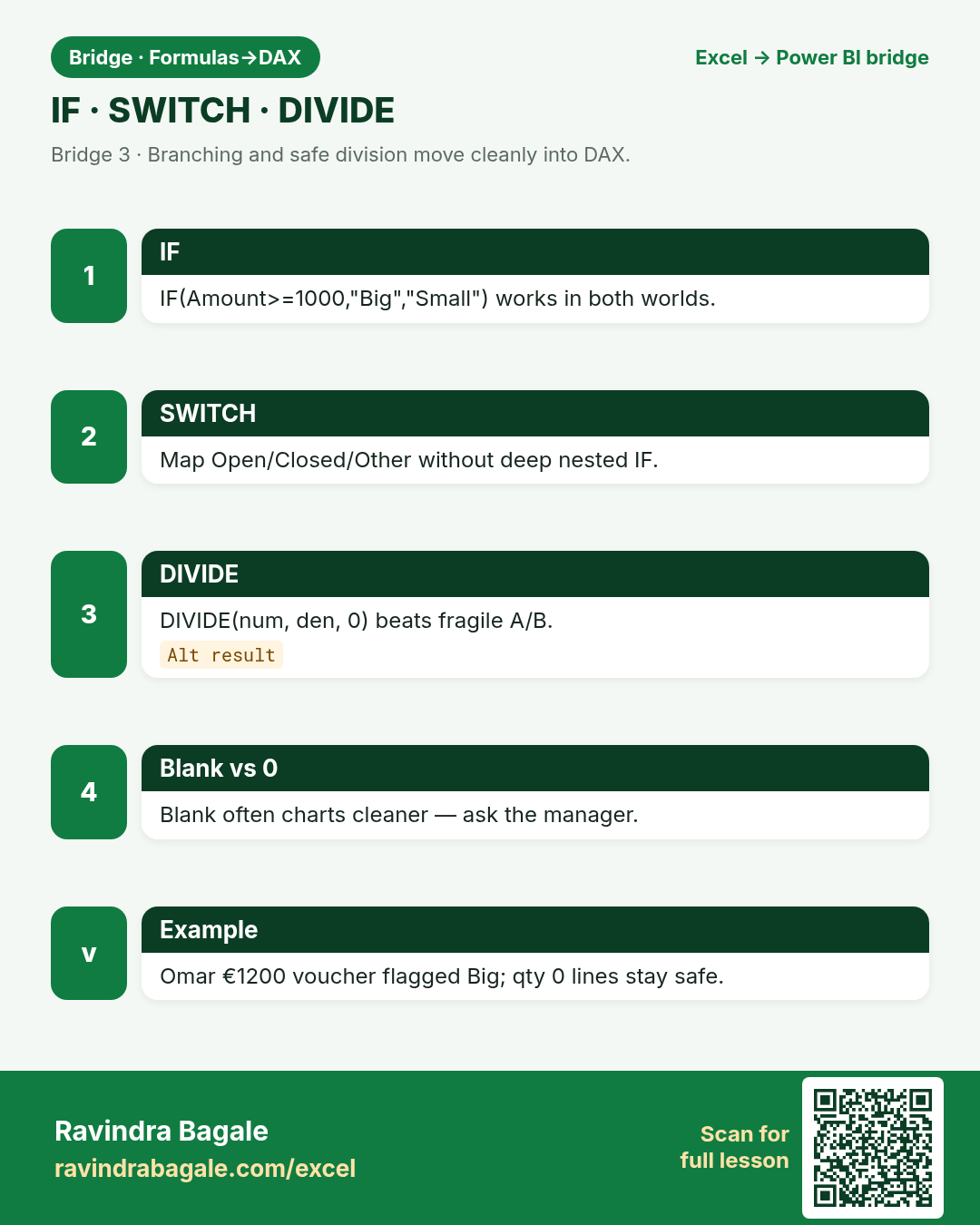
- Excel: =IF(B2>=1000,"Big","Small").
- DAX measure/column: IF(Sales[Amount]>=1000, "Big", "Small").
- Excel nested IF for status colours → DAX SWITCH(Tickets[Status], "Open","Needs work", "Closed","Done", "Other").
- Keep labels short for visuals and cards.
| Excel | Power BI / DAX | Result | Meaning |
|---|---|---|---|
Excel=IF(Amount>=1000,"Big","Small") |
DAXIF(Sales[Amount]>=1000, "Big", "Small") |
Big |
Omar’s €1200 Dubai desk voucher flagged Big. |
6. AVERAGEIF → AVERAGEX / CALCULATE(AVERAGE)
Friends,
Always name the measure with the grain: Average Wait (mins) — not just Average.
चला मित्रांनो
Measure ला grainसह नाव द्या: Average Wait (mins) — फक्त Average नाही.
चलो दोस्तों
Measure का नाम grain के साथ: Average Wait (mins) — सिर्फ़ Average नहीं.
Why: Conditional averages appear in healthcare wait times and delivery fees.
What: CALCULATE(AVERAGE(...), filters) or AVERAGEX over a filtered table.
How:
- Excel: =AVERAGEIF(City,"Kolhapur",WaitMins).
- DAX: CALCULATE(AVERAGE(Visits[WaitMins]), Visits[City]="Kolhapur").
- For “average of a row-by-row expression”, learn AVERAGEX later.
- Watch blanks: AVERAGE in DAX skips blanks like Excel usually does.
| Excel | Power BI / DAX | Result | Meaning |
|---|---|---|---|
Excel=AVERAGEIF(City,"Kolhapur",WaitMins) |
DAXCALCULATE(AVERAGE(Visits[WaitMins]), Visits[City]="Kolhapur") |
18 mins |
Neha’s Kolhapur clinic average wait. |
7. Safe division (IF / IFERROR → DIVIDE)
Friends,
Blank often charts cleaner than zero. Ask what the manager should see.
चला मित्रांनो
चार्टसाठी Blank अनेकदा zero पेक्षा स्वच्छ. मॅनेजरला काय दिसले पाहिजे ते विचारा.
चलो दोस्तों
चार्ट के लिए Blank अक्सर zero से साफ़. मैनेजर को क्या दिखे पूछो.
Why: Division by zero breaks dashboards. Excel uses IF or IFERROR; DAX has DIVIDE.
What: DIVIDE(numerator, denominator, alternate_result).
How:
- Excel habit: =IF(B2=0,0,A2/B2) or IFERROR(A2/B2,0).
- DAX: DIVIDE(SUM(Sales[Amount]), SUM(Sales[Qty]), 0).
- Prefer DIVIDE over manual IF for readability.
- Decide if alternate should be BLANK() (better for charts) or 0.
| Excel | Power BI / DAX | Result | Meaning |
|---|---|---|---|
Excel=IF(Qty=0,0,Amount/Qty) |
DAXDIVIDE(SUM(Sales[Amount]), SUM(Sales[Qty]), 0) |
₹250 |
Unit price style metric for Pune lines with qty > 0. |
8. Text joins and case (LibreOffice-safe habits)
Friends,
Clean early in Power Query. DAX should calculate, not mop floors.
चला मित्रांनो
Power Query मध्ये लवकर स्वच्छ करा. DAX ने मोजावे, फरशी पुसू नये.
चलो दोस्तों
Power Query में जल्दी साफ़ करो. DAX को नापना है, फर्श नहीं पोछना.
Why: You still clean text. Power Query does most cleaning; DAX has UPPER/LOWER/LEFT too.
What: Prefer Power Query for cleaning; use DAX text functions sparingly on measures/columns.
How:
- Excel class-safe join: =A2 & " - " & B2 (avoid TEXTJOIN in LibreOffice checks).
- DAX: Sales[City] & " - " & Sales[Status] in a calculated column if needed.
- Case: UPPER / LOWER / PROPER-style cleaning is happier in Power Query.
- Do not build giant text report columns in DAX when a visual label will do.
| Excel | Power BI / DAX | Result | Meaning |
|---|---|---|---|
Excel=A2 & " - " & B2 |
DAXSales[City] & " - " & Sales[Status] |
Pune - Delivered |
Label for a detail table — still prefer PQ for heavy cleans. |
9. Why the same measure changes on a visual
Friends,
About this data must say which currency a total uses. Never sum ₹ and € as one number.
चला मित्रांनो
About this data मध्ये currency सांगा. ₹ आणि € एकत्र SUM करू नका.
चलो दोस्तों
About this data में currency लिखो. ₹ और € को एक SUM मत बनाओ.
Why: Students panic when Total Sales shows different numbers in two cards. That is filter context, not a bug.
What: Slicers, rows of a matrix, and page filters all shape CALCULATE.
How:
- Put [Total Amount] on a card — sees all data (unless page filters).
- Put the same measure on a matrix with City on rows — each row filters City.
- Excel parallel: a PivotTable value changes per row label.
- CALCULATE adds or replaces filters on top of that context.
| Excel | Power BI / DAX | Result | Meaning |
|---|---|---|---|
Excel PivotSum of Amount by City |
PBI MatrixSame measure [Total Amount] + City on rows |
Per city |
Manchester £ and Pune ₹ rows can sit in one model with a currency column — do not blindly sum mixed currency. |
10. Pocket cheat sheet (print this card later)
Friends,
Master five. Then open CALCULATE with ALL / time intelligence in the Power BI DAX chapters.
चला मित्रांनो
पाच वर प्रभुत्व. मग Power BI DAX chapters मध्ये ALL / time intelligence.
चलो दोस्तों
पाँच पर महारत. फिर Power BI DAX chapters में ALL / time intelligence.
Why: A short map beats a long book on day one.
What: Highest-traffic Excel → DAX replacements.
How:
- SUM / SUMIF(S) → SUM + CALCULATE
- COUNT / COUNTIF(S) → COUNTROWS + CALCULATE
- AVERAGEIF → CALCULATE(AVERAGE(...), ...)
- IF → IF; nested status maps → SWITCH
- VLOOKUP/XLOOKUP → relationship + RELATED (or visual fields)
- A/B with zero risk → DIVIDE
- Helper columns forever → ask if a measure is enough
| Excel | Power BI / DAX | Result | Meaning |
|---|---|---|---|
Excel comfortSUMIFS + VLOOKUP + IF |
DAX starter kitSUM, CALCULATE, RELATED, IF, DIVIDE |
Enough |
Chen Wei’s Singapore demo pack runs on these five. |
Practice tasks (12)
Use bridge-dax-practice.xlsx. Excel side must run in LibreOffice: avoid XLOOKUP, TEXTJOIN, TEXTSPLIT. DAX column is written as text for Desktop practice.
- On Sales sheet, write Excel Total Amount with SUM (LibreOffice-safe).
Hint
Simple =SUM(Amount column).
- Write Excel SUMIFS for City=Pune.
Hint
=SUMIFS(Amount,City,"Pune")
- Write Excel SUMIFS for City=Nashik and Status=Delivered.
Hint
Two criteria SUMIFS.
- Write COUNTIFS for Status=Open and City=Hyderabad on Tickets.
Hint
Open + Hyderabad.
- Simulate a lookup: VLOOKUP ProductID into ProductName (range lookup FALSE).
Hint
Product sheet columns A:B.
- Add IF flag Big/Small for Amount>=1000.
Hint
=IF(Amount>=1000,"Big","Small")
- Use IF to protect division Amount/Qty when Qty=0.
Hint
=IF(Qty=0,0,Amount/Qty)
- On DAX_Translate, fill the DAX column for each Excel formula (words + code).
Hint
Use chapter examples.
- Explain in one sentence why RELATED needs a relationship.
Hint
Write on Notes sheet.
- Mark which rows are mixed-currency risks before any total.
Hint
Currency column — ₹ vs €.
- AVERAGEIF wait mins for Kolhapur on Visits.
Hint
=AVERAGEIF(City,"Kolhapur",WaitMins)
- Rewrite nested IF status labels as a SWITCH plan on paper (Open/Closed/Other).
Hint
Three-line SWITCH sketch.
Quick quiz
Q1. Best first DAX habit for totals?
Q2. SUMIFS maps most closely to…
Q3. Preferred replacement for most VLOOKUP name pulls?
Q4. DIVIDE is mainly for…
Q5. SWITCH is happier than deep nested IF when…
Q6. Same measure, different number on two visuals — often because of…
Q7. COUNTIFS open tickets in one city becomes…
Q8. Before summing Amount across Pune and Berlin rows you must…
Loading practice tasks...
- Rows in the fact table (Easy): How many orders are in the Sales table?
- Total amount (Easy): Add up the Amount column of Sales.
- Total quantity (Easy): Add up the Qty column of Sales.
- Products in the dimension (Easy): How many products are in the Products table?
- Products actually sold (Medium): How many of the 5 Product IDs (P01 to P05) appear at least once in Sales?
- Amount for one city (Medium): Add up Amount where City is "London".
- Product name through the relationship (Medium): What is the Product name for Product ID "P03"?
- Sales of one product (Medium): Add up Amount where Product ID is "P03".
- Average order amount (Medium): Find the average Amount, rounded to 0 decimals.
- Category of the first order (Hard): Find the Category of the product in the first order.
- Biggest order in London (Hard): What is the largest Amount where City is "London"?
- Share of P03 (Hard): What share of the total Amount comes from Product ID "P03"? Round to 3 decimals.
Quick revision cards (3)
Approved Excel card style: standalone, no tip/photo section, QR to this lesson.