Excel TAKE Function
Chala mitrano — today TAKE. Grab the first 3 rows — or the last 2 with a negative.
चला मित्रांनो — आज TAKE. पहिल्या 3 rows घ्या — किंवा negative ने शेवटच्या 2.
चलो दोस्तों — आज TAKE. पहली 3 rows लो — या negative से आखिरी 2.
Purpose
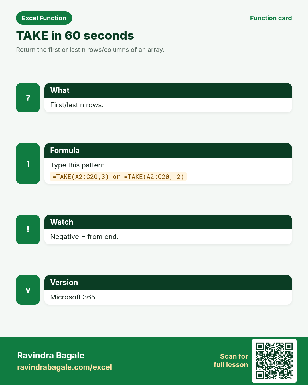
Return the first or last n rows/columns of an array.
Return value
A spilled subset from the start or end.
Syntax
Arguments
| Argument | Required? | Description |
|---|---|---|
array | Required | Source array. |
rows | Required | How many rows from top (negative = from bottom). |
columns | Optional | How many columns from left (negative = from right). |
Version
Microsoft 365. Not in perpetual Excel 2019 without dynamic arrays. Sheets has partial cousins.
How to use — Why → What → How
Why: Dashboards often show top-n only. TAKE slices without helper rows. Top-n previews for Nashik dashboards and Toronto packs. In Indian back offices and foreign sister teams, TAKE shows up on live dashboards and spill ranges every week.
What: TAKE keeps the first rows (or last if rows is negative). Same idea for columns. Read every argument in the table once before you type; each one changes the answer on purpose.
How — numbered steps:
- Type =TAKE(A2:C20,3).
- =TAKE(A2:C20,-2) for last two rows.
- Pair with SORT for top scores.
Ravindra Bagale's Tip
Friends, after TAKE, find one column or range in a real workbook this week where this lesson saves time.
Ravindra Bagale's Tip – मराठी
मित्रांनो, TAKE नंतर या आठवड्यात खरी workbook मधील एक संख्या column सुधारा.
Ravindra Bagale's Tip – हिंदी
दोस्तों, TAKE के बाद इस हफ़्ते असली workbook का एक संख्या column सुधारो.
Ravindra Bagale's Tip
Friends, sleep on TAKE; rebuild example 1 tomorrow without looking.
Ravindra Bagale's Tip – मराठी
मित्रांनो, TAKE वर झोपा; उद्या उदाहरण 1 न पाहता लिहा.
Ravindra Bagale's Tip – हिंदी
दोस्तों, TAKE पर सोकर कल उदाहरण 1 बिना देखे लिखो.
Ravindra Bagale's Tip
Friends, say the business question in plain words before =TAKE.
Ravindra Bagale's Tip – मराठी
मित्रांनो, =TAKE आधी व्यवसाय प्रश्न साध्या शब्दांत सांगा.
Ravindra Bagale's Tip – हिंदी
दोस्तों, =TAKE से पहले व्यवसाय प्रश्न सादे शब्दों में बोलो.
Ravindra Bagale's Tip
Friends, check a known case with a calculator before you trust a long TAKE chain.
Ravindra Bagale's Tip – मराठी
मित्रांनो, लांब TAKE chain वर विश्वास ठेवण्यापूर्वी कॅल्क्युलेटरने एक ज्ञात case तपासा.
Ravindra Bagale's Tip – हिंदी
दोस्तों, लंबी TAKE chain पर भरोसा करने से पहले कैलकुलेटर से एक जाना हुआ case जाँचो.
Ravindra Bagale's Tip
Friends, after you finish TAKE, open yesterday’s real workbook and find one place this function would have saved ten minutes.
Ravindra Bagale's Tip – मराठी
मित्रांनो, TAKE नंतर कालची खरी वर्कबुक उघडा आणि शोधा जिथे हे फंक्शन दहा मिनिटे वाचवू शकले असते.
Ravindra Bagale's Tip – हिंदी
दोस्तों, TAKE के बाद कल की असली वर्कबुक खोलो और ढूँढो जहाँ यह फ़ंक्शन दस मिनट बचा सकता था.
Ravindra Bagale's Tip
Friends, treat TAKE like a seatbelt on spill ranges — clear #SPILL! blocks first.
Ravindra Bagale's Tip – मराठी
मित्रांनो, TAKE ला spill ranges वरील seatbelt समजा — आधी #SPILL! साफ करा.
Ravindra Bagale's Tip – हिंदी
दोस्तों, TAKE को spill ranges पर seatbelt समझो — पहले #SPILL! साफ़ करो.
Download practice file: practice-take.xlsx (includes sheet About this data, practice sheets, and Answers).
Worked examples
1) First 2
Nashik.
| Name | Marks |
|---|---|
| Asha | 72 |
| Ben | 90 |
| Cid | 85 |
Result: {Asha,72;Ben,90}
What it means: Top two rows.
2) Last 1
Tail.
| Name |
|---|
| Asha |
| Ben |
| Cid |
Result: {Cid}
What it means: Last row.
3) Toronto $
Fees.
| $ |
|---|
| 10 |
| 20 |
| 30 |
| 40 |
Result: {10;20;30}
What it means: First three.
4) Columns
Left 1.
| A | B |
|---|---|
| 1 | 9 |
| 2 | 8 |
Result: {1;2}
What it means: First column only.
5) With SORT
Top score row.
| Name | Marks |
|---|---|
| Asha | 72 |
| Ben | 90 |
Result: {Ben,90}
What it means: Best row.
6) Too many
Clamp.
| X |
|---|
| 1 |
| 2 |
Result: {1;2}
What it means: Returns all available.
Common errors and fixes
Notes and tips
- Revisit the TAKE errors table after the quiz.
- Build example 1 from memory on a blank sheet.
- Check number vs text if a result looks wrong.
- Teach one tip in Marathi or Hindi this week.
- Keep currency symbols consistent inside one report column (practice mixes ₹ $ £ €).
- Drill: TAKE first two of a three-row name list from memory.
- TAKE vs INDEX: spill a block versus one cell.
- Fictional sample data only — names and amounts are for learning.
- Print the TAKE revision card for one week of real worksheets.
- Ask juniors to predict before they press Enter.
- Track your top mistake with this function monthly.
- Top-n previews for Nashik dashboards and Toronto packs.
- Interview tip: explain the business question before the formula.
- Classroom drill: invent three brand-new formulas from your city without the page open.
- If a result looks wrong, check blanks vs zeros before rewriting.
- When Excel versions differ, note the LibreOffice / Sheets fallback in a cell comment.
- Prefer clear ranges over whole-column refs on huge sheets if speed matters.
- Document units (₹, kg, days) in the header so totals stay honest.
- Print the revision card for TAKE for one week of real worksheets.
- When helping a junior, ask them to predict before Enter.
- Share one tip with a classmate in Marathi or Hindi.
- Keep currency symbols consistent inside a single report column.
- Interview tip: explain the business question before the formula.
- If a result looks wrong, check spill range blocks (#SPILL!) before rewriting.
- When Excel versions differ, write a LibreOffice / Sheets fallback under a comment.
In real work
Drill: TAKE first two of a three-row name list from memory. Top-n previews for Nashik dashboards and Toronto packs. Classroom drill: write three brand-new TAKE formulas on a blank sheet using names from your own city — if you can invent them without the page open, you own the skill. Then break one formula on purpose and watch the error; recovering from that break is half of interview readiness. Always verify with a known case before trusting a long chain. Keep a personal notebook of the one mistake you make most often with this function; review it monthly.
How it compares
TAKE vs INDEX: spill a block versus one cell.
Interview corner
- Negative rows?
- From bottom.
- vs DROP?
- Keep vs remove.
- Too many?
- Returns all.
Related functions
DROP, CHOOSEROWS, INDEX, FILTER
Practice tasks (10)
- Task 1. First 2 rows.TAKE.
- Task 2. Last row −1.Tail.
- Task 3. First 3 fees.$.
- Task 4. Left column.Cols.
- Task 5. TAKE SORT top.Best.
- Task 6. Interview.Talk.
- Task 7. Teach.Teach.
- Task 8. Clamp demo.All.
- Task 9. Fill.Fill.
- Task 10. Document.Note.
Quick quiz
Answers: Q1=Last row, Q2=Top two, Q3=Yes, Q4=All available, Q5=TAKE(SORT(...),1) (check after you try).
Revision card
Standalone card (no tip or photo strip). QR opens this lesson. Download the PNG and revise offline.