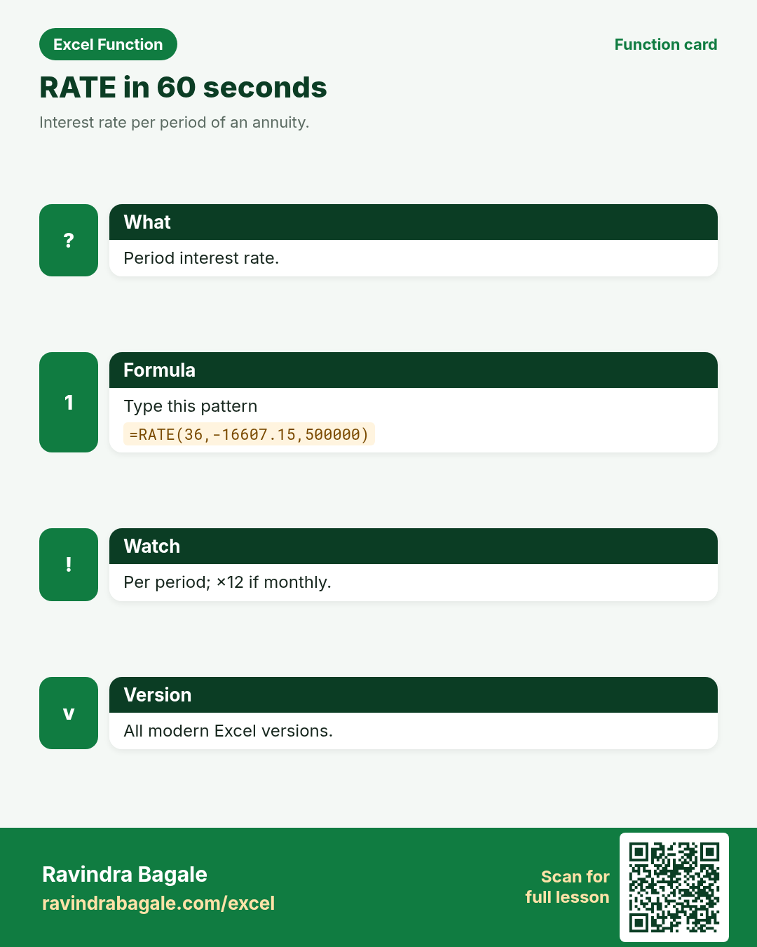
Excel RATE Function
Chala mitrano — today RATE. What rate makes this EMI and principal fit?
चला मित्रांनो — आज RATE. कोणता दर या EMI आणि मुद्दलाला जुळवतो?
चलो दोस्तों — आज RATE. कौन सा दर इस EMI और मूलधन को मिलाता है?
Purpose
Interest rate per period of an annuity.
Return value
The rate per period (multiply by 12 for nominal annual if monthly).
Syntax
Arguments
| Argument | Required? | Description |
|---|---|---|
nper | Required | Periods. |
pmt | Required | Payment. |
pv | Required | Present value. |
fv | Optional | Future value. |
type | Optional | 0 or 1. |
guess | Optional | Starting guess (default 10%). |
Version
All modern Excel versions. LibreOffice Calc and Google Sheets have matching functions (names may vary slightly).
How to use — Why → What → How
Why: When the bank quote feels odd, RATE reverse-engineers the period rate. Implied-rate checks for Indore dealers and Boston lenders.
What: RATE uses iteration. Returns rate per period — ×12 for a nominal annual percentage on monthly models. In practice, keep the rate and nper in the same unit — annual rate with monthly payments means rate/12 and nper×12. Mixing units is the most common silent error: Excel returns a number that looks plausible but is wrong for the loan. Sign convention: money you receive is positive; money you pay out is negative. For a borrower, PV is positive and PMT is negative. Build amortization with PMT for the installment, IPMT/PPMT for each period’s split, and CUMIPMT/CUMPRINC for year totals.
How — numbered steps:
- Type =RATE(36,-16607.15,500000).
- Expect ~1% monthly → 12% nominal.
- Provide guess if it fails to converge.
Ravindra Bagale's Tip
Friends, after RATE, find one column or range in a real workbook this week where this lesson saves time.
Ravindra Bagale's Tip – मराठी
मित्रांनो, RATE नंतर या आठवड्यात खरी workbook मधील एक संख्या column सुधारा.
Ravindra Bagale's Tip – हिंदी
दोस्तों, RATE के बाद इस हफ़्ते असली workbook का एक संख्या column सुधारो.
Ravindra Bagale's Tip
Friends, sleep on RATE; rebuild example 1 tomorrow without looking.
Ravindra Bagale's Tip – मराठी
मित्रांनो, RATE वर झोपा; उद्या उदाहरण 1 न पाहता लिहा.
Ravindra Bagale's Tip – हिंदी
दोस्तों, RATE पर सोकर कल उदाहरण 1 बिना देखे लिखो.
Ravindra Bagale's Tip
Friends, say the business question in plain words before =RATE.
Ravindra Bagale's Tip – मराठी
मित्रांनो, =RATE आधी व्यवसाय प्रश्न साध्या शब्दांत सांगा.
Ravindra Bagale's Tip – हिंदी
दोस्तों, =RATE से पहले व्यवसाय प्रश्न सादे शब्दों में बोलो.
Ravindra Bagale's Tip
Friends, check a known case with a calculator before you trust a long RATE chain.
Ravindra Bagale's Tip – मराठी
मित्रांनो, लांब RATE chain वर विश्वास ठेवण्यापूर्वी कॅल्क्युलेटरने एक ज्ञात case तपासा.
Ravindra Bagale's Tip – हिंदी
दोस्तों, लंबी RATE chain पर भरोसा करने से पहले कैलकुलेटर से एक जाना हुआ case जाँचो.
Ravindra Bagale's Tip
Friends, after you finish RATE, open yesterday’s real workbook and find one place this function would have saved ten minutes.
Ravindra Bagale's Tip – मराठी
मित्रांनो, RATE नंतर कालची खरी वर्कबुक उघडा आणि शोधा जिथे हे फंक्शन दहा मिनिटे वाचवू शकले असते.
Ravindra Bagale's Tip – हिंदी
दोस्तों, RATE के बाद कल की असली वर्कबुक खोलो और ढूँढो जहाँ यह फ़ंक्शन दस मिनट बचा सकता था.
Ravindra Bagale's Tip
Friends, treat RATE sign carefully — positive PV usually means negative payment outflow.
Ravindra Bagale's Tip – मराठी
मित्रांनो, RATE चा sign काळजीपूर्वक पाहा — positive PV म्हणजे सहसा negative payment outflow.
Ravindra Bagale's Tip – हिंदी
दोस्तों, RATE का sign सावधानी से देखो — positive PV का मतलब आमतौर पर negative payment outflow.
Download practice file: practice-rate.xlsx (includes sheet About this data, practice sheets, and Answers).
Worked examples
1) Monthly rate
Indore.
| # |
|---|
Result: 0.01
What it means: 1% per month.
2) Annual nominal
×12.
| # |
|---|
Result: 0.12
What it means: 12% nominal.
3) Boston $
Car.
| # |
|---|
Result: 0.005
What it means: 0.5%/mo → 6% nominal.
4) Savings
FV goal.
| # |
|---|
Result: 0.006667
What it means: ~0.6667%/mo (~8% yr).
5) Guess
Help converge.
| # |
|---|
Result: 0.01
What it means: Same with guess.
6) #NUM!
No converge.
| # |
|---|
Result: #NUM!
What it means: Impossible / need guess.
Common errors and fixes
Notes and tips
- Revisit the RATE errors table after the quiz.
- Build example 1 from memory on a blank sheet.
- Check number vs text if a result looks wrong.
- Teach one tip in Marathi or Hindi this week.
- Keep currency symbols consistent inside one report column (practice mixes ₹ $ £ €).
- Drill: recover 1% monthly from the ₹5L EMI numbers.
- RATE vs RRI: annuity with payments versus two-value growth.
- Fictional sample data only — names and amounts are for learning.
- Print the RATE revision card for one week of real worksheets.
- Ask juniors to predict before they press Enter.
- Track your top mistake with this function monthly.
- Implied-rate checks for Indore dealers and Boston lenders.
- Interview tip: explain the business question before the formula.
- Classroom drill: invent three brand-new formulas from your city without the page open.
- If a result looks wrong, check blanks vs zeros before rewriting.
- When Excel versions differ, note the LibreOffice / Sheets fallback in a cell comment.
- Prefer clear ranges over whole-column refs on huge sheets if speed matters.
- Document units (₹, kg, days) in the header so totals stay honest.
- Print the revision card for RATE for one week of real worksheets.
- When helping a junior, ask them to predict before Enter.
- Share one tip with a classmate in Marathi or Hindi.
- Keep currency symbols consistent inside a single report column.
- When Excel versions differ, write a LibreOffice / Sheets fallback under a comment.
- Keep rate and nper units matched (monthly with monthly) or the EMI will silently mislead.
- Document whether the sheet is borrower’s view (PV>0 → PMT<0) or lender’s view.
- Round displayed EMI with ROUND(...,2) for client letters; keep full precision in calc columns.
- For RATE/IRR #NUM!, supply a guess near 0.1 when cash-flow signs flip more than once.
- Pair NPV with a separate time-0 outflow cell — do not bury the initial invest inside values[1] by accident.
- Fictional EMI and cash-flow figures only — never paste real customer loan data into class files.
- Compare your EMI to a bank quote: if off by a lot, you forgot /12; if off by paisa, rounding.
- Teach one junior the sign convention in Marathi or Hindi this week — teaching locks it.
In real work
Drill: recover 1% monthly from the ₹5L EMI numbers. Implied-rate checks for Indore dealers and Boston lenders. Classroom drill: write three brand-new RATE formulas on a blank sheet using names from your own city — if you can invent them without the page open, you own the skill. Then break one formula on purpose and watch the error; recovering from that break is half of interview readiness. Always verify with a known case before trusting a long chain. Keep a personal notebook of the one mistake you make most often with this function; review it monthly. Excel’s financial engine uses the same closed-form annuity formulas taught in CFA Level I. PMT isolates the constant installment; IPMT the interest slice; PPMT the principal residual — and PMT = IPMT + PPMT for each period when FV and type match. NPV discounts values starting at period 1, so keep the time-0 investment outside the values array. XNPV/XIRR need actual dates; RRI inverts growth between two pots; EFFECT/NOMINAL bridge stated APR and true EAR under m compounding periods. Bank EMI sheets often round each installment to two decimals — expect ₹0.01–₹0.05 drift versus raw Excel PMT on long tenures.
How it compares
RATE vs RRI: annuity with payments versus two-value growth.
Interview corner
- Returns?
- Rate per period.
- Annualise?
- × periods/year.
- #NUM!?
- Guess or fix signs.
Related functions
Practice tasks (10)
- Task 1. RATE monthly.1%.
- Task 2. ×12 nominal.12%.
- Task 3. $ car RATE.Boston.
- Task 4. SIP RATE.8% yr.
- Task 5. Force #NUM!.Bad.
- Task 6. Interview.Talk.
- Task 7. Teach.Teach.
- Task 8. Use guess.Guess.
- Task 9. Fill.Fill.
- Task 10. Document.Note.
Quick quiz
Answers: Q1=~1%/mo, Q2=×12, Q3=#NUM!, Q4=Annuity rate vs growth between two values, Q5=10% (check after you try).
Revision card
Standalone card (no tip or photo strip). QR opens this lesson. Download the PNG and revise offline.