Excel chart chooser — what do you want to show?
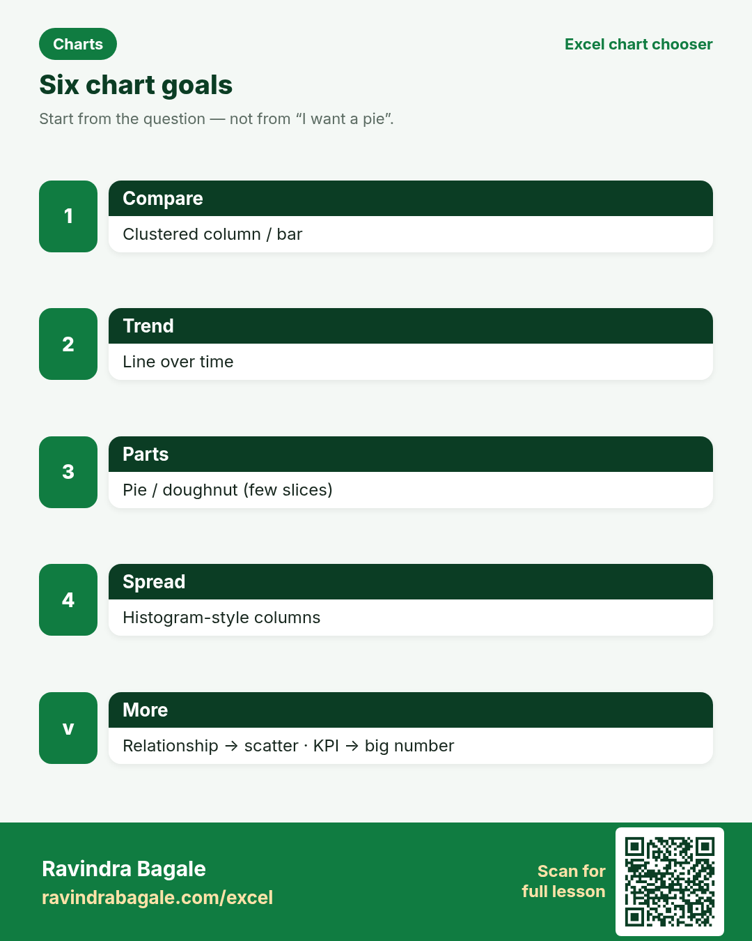
Friends, do not start with “I want a pie.” Start with the question. This page maps six questions to a chart.
चला मित्रांनो — “मला pie हवा” असे सुरू करू नका. प्रश्नाने सुरू करा. सहा प्रश्नांसाठी चार्ट.
चलो दोस्तों — “मुझे pie चाहिए” से शुरू मत करो। सवाल से शुरू करो। छह सवालों के लिए चार्ट।
excel/chart-chooser/. Linked lessons: Chapter 8 and 8-12 Choosing the right chart.Why this page
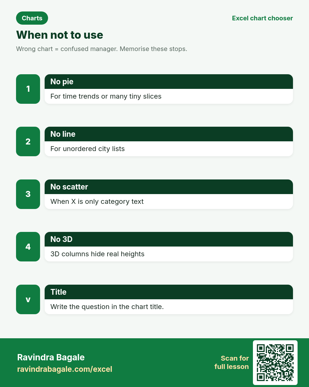
Why: Wrong charts confuse managers. A pie of monthly sales hides the trend. A line of five unordered cities invents a fake journey.
What: Six goals. Each block has a recommended chart, a when-not-to-use note, a sample image, and How steps.
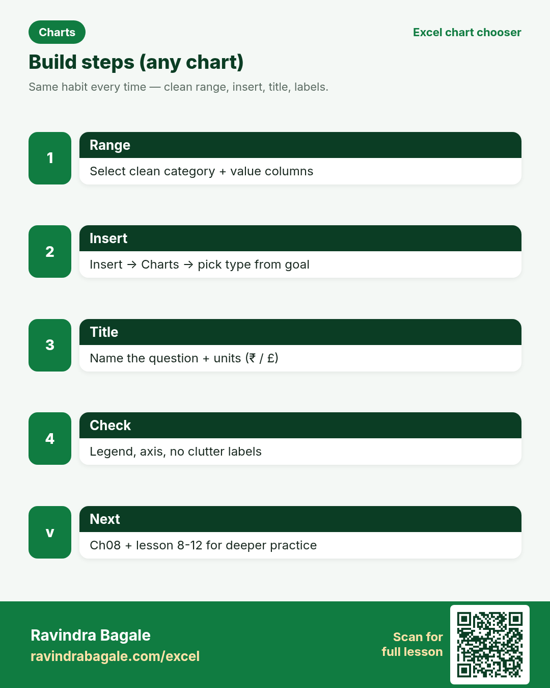
How: Jump to your goal below. Build the chart in Excel. Then try the practice tasks and quiz.
Ravindra Bagale's Tip
Friends, write the question in the chart title. “Orders by city — 2025 vs 2026” beats “Chart 1”.
Ravindra Bagale's Tip – मराठी
मित्रांनो, चार्ट title मध्ये प्रश्न लिहा. “Orders by city” हे “Chart 1” पेक्षा चांगले.
Ravindra Bagale's Tip – हिंदी
दोस्तों, चार्ट title में सवाल लिखो। “Orders by city” बेहतर है “Chart 1” से।
What do you want to show?
Compare values side by side
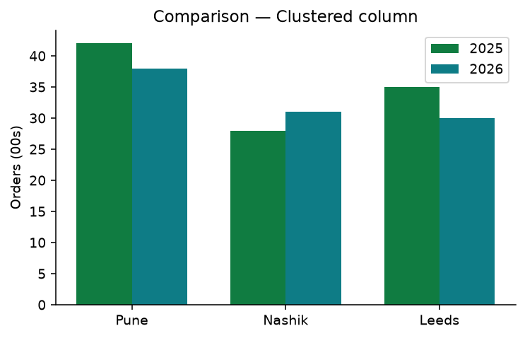
Recommended: Clustered column (or bar)Why: Managers ask which city or product is higher. Columns make height easy to compare.
What: Categories on the axis; one or more series as columns.
How — numbered steps:
- Select category + value columns.
- Insert → Charts → Clustered Column.
- Add a clear chart title (example: Orders by city).
- If two years, add both value columns before Insert.
- Keep gap width readable; avoid 3D columns.
Example: Priya Sharma (Pune) compares 2025 vs 2026 order volume for Pune, Nashik and Leeds.
What do you want to show?
Show change over time
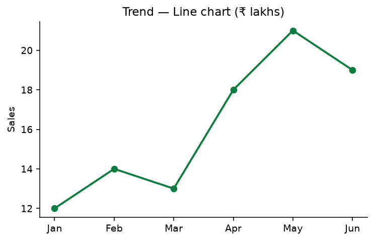
Recommended: Line chart (or column for few periods)Why: Trends answer “are we going up or down?” Lines guide the eye across months.
What: Time on the horizontal axis; measure on the vertical axis.
How — numbered steps:
- Put months in one column, values next to them.
- Select the range → Insert → Line with markers.
- Title: Sales trend (₹ lakhs).
- Add a thin target line manually if needed (optional series).
- Check that dates/months are sorted.
Example: Omar Hassan (Dubai desk using ₹ training file) plots Jan–Jun sales for leadership.
What do you want to show?
Show parts of a whole
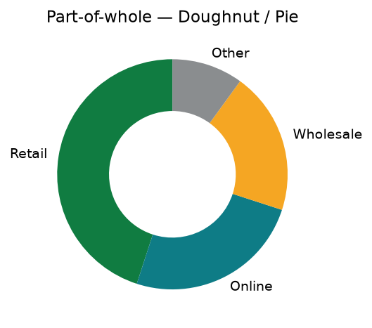
Recommended: Pie or doughnut (few slices)Why: Share-of-total questions (“how much is retail?”) fit part-of-whole charts.
What: One whole = 100%. Each slice is a category’s share.
How — numbered steps:
- Build a small summary: Category | Amount.
- Insert → Pie or Doughnut.
- Show percentages in data labels.
- Order slices largest to smallest.
- If many categories, switch to bar.
Example: James Cole (Birmingham) shows channel mix: Retail, Online, Wholesale, Other.
What do you want to show?
Show how values are spread
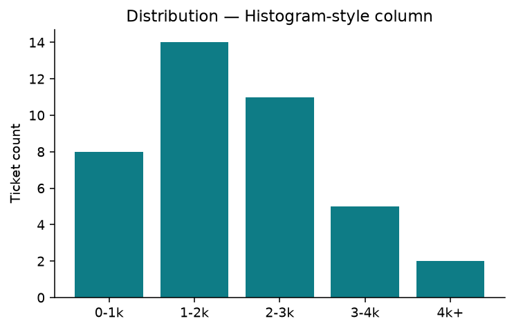
Recommended: Histogram-style column (or box plot add-in)Why: Distribution answers “are most tickets small or large?” — not just the average.
What: Buckets (bins) on the axis; count of rows in each bucket.
How — numbered steps:
- Create bin labels (0–1k, 1–2k…).
- COUNTIF / FREQUENCY into a count column.
- Insert Clustered Column.
- Title: Ticket size distribution.
- Or use Excel’s Histogram chart if available in your build.
Example: Ananya Joshi (support, Pune) bins ticket values to see if refunds cluster under ₹2,000.
What do you want to show?
Show relationship between two numbers
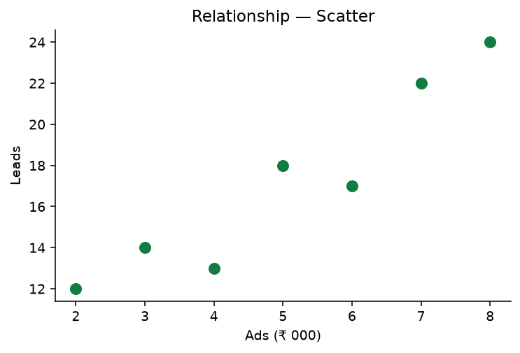
Recommended: Scatter (X‑Y)Why: Relationship questions: “when ads rise, do leads rise?” Scatter plots pairs of numbers.
What: One measure on X, another on Y; each point is a row.
How — numbered steps:
- Two numeric columns (Ads, Leads).
- Select both → Insert → Scatter.
- Add axis titles with units (₹ 000, leads).
- Optional: add a trendline (Chart Design).
- Check outliers before presenting.
Example: Sofia Keller (Berlin marketing) plots ads spend vs leads for weekly reviews.
What do you want to show?
Highlight one key number
Recommended: KPI card / single big number (or gauge carefully)Why: Leaders often need one headline metric before details — on-time %, NPS, cash.
What: A large number, short label, optional target comparison.
How — numbered steps:
- Compute the KPI in a cell (example: on-time deliveries / total).
- Format as percentage.
- Place it large on a dashboard sheet (font 28–36).
- Optional: sparkline beside it for trend.
- Link to detail charts below.
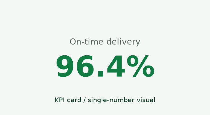
Example: Ravindra’s sample logistics card: 96.4% on-time delivery for the week.
Practice tasks (12)
- Task 1. Build a clustered column for three cities × two years.Hint: Comparison block
- Task 2. Make a 6-month line chart titled with units.Hint: Trend block
- Task 3. Create a doughnut with four channels; show % labels.Hint: Part-of-whole
- Task 4. Explain why a pie is a bad monthly sales trend chart.Hint: time ≠ slices
- Task 5. Bin 20 ticket amounts into 5 buckets and chart counts.Hint: Distribution
- Task 6. Plot ads vs leads on a scatter; add axis titles.Hint: Relationship
- Task 7. Design a KPI cell for on-time % with large font.Hint: KPI block
- Task 8. Take a wrong pie you find online and rewrite which chart fits.Hint: use the six goals
- Task 9. Open Ch 8 lesson 8-12 and list two tips that match this page.Hint: sidebar link
- Task 10. Rebuild the comparison chart as horizontal bars for long city names.Hint: bar vs column
- Task 11. Add data labels only where they help (not on every scatter point).Hint: reduce clutter
- Task 12. Bonus: one dashboard sheet with KPI + trend + comparison.Hint: Ch 13 dashboards
Quick quiz
Answers: column, line, few slices, two numbers, one headline, distribution, True, False
Revision cards
Three standalone cards. QR opens this chart chooser. Card images are on S3 under excel/chart-chooser/.