Chapter 32 Free
32. Cleaning Dirty Data in Excel
Friends, dirty data is normal. CSVs from shops, banks, clinics, IT desks and lorries arrive with spaces, text numbers, odd dates and duplicate rows. In this chapter we clean each mess with Why → What → How, easy examples, a practice workbook, and Power Query for the weekly repeat.
मित्रांनो, dirty data सामान्य आहे. दुकान, बँक, क्लिनिक, IT desk आणि वाहतूक यांच्या CSV मध्ये spaces, text numbers, विचित्र dates आणि duplicate rows येतात. या chapter मध्ये आपण प्रत्येक गोंधळ Why → What → How ने साफ करतो.
दोस्तों, dirty data आम बात है. दुकान, बैंक, क्लिनिक, IT desk और लॉजिस्टिक्स की CSV में spaces, text numbers, अजीब dates और duplicate rows आते हैं. इस चैप्टर में हम हर गड़बड़ Why → What → How से साफ़ करते हैं.
At deploy, files go to s3://ravindrabagale-cards/excel/dirty-data/ (public S3 downloads).
What you will learn
- Spot every common dirty-data pattern in real exports.
- Fix them with formulas (LibreOffice-safe fallbacks) and with menus.
- Use Power Query so Monday’s cleanup refreshes itself.
- Document rules on an About sheet so juniors do not guess.
A Monday morning story
Priya’s Pune kirana CSV, Omar’s Dubai bank desk sheet, Ananya’s Hyderabad IT tickets and Sofia’s Berlin lane weights all land in one inbox. Your manager asks for one Pivot by city before lunch. This chapter is the cleaning path that makes that Pivot honest.
Ravindra Bagale’s Tip
Clean in this order: (1) spaces/hidden chars (2) types and dates (3) split units/currency (4) categories and codes (5) duplicates (6) outliers (7) shape wide→tall. Skipping order creates new bugs.
Ravindra Bagale’s Tip – मराठी
हा क्रम ठेवा: (1) spaces/hidden (2) types व dates (3) units/currency split (4) categories/codes (5) duplicates (6) outliers (7) wide→tall. क्रम सोडला की नवे bugs येतात.
Ravindra Bagale’s Tip – हिंदी
यह क्रम रखें: (1) spaces/hidden (2) types और dates (3) units/currency split (4) categories/codes (5) duplicates (6) outliers (7) wide→tall. क्रम छोड़ोगे तो नए bugs आएँगे.
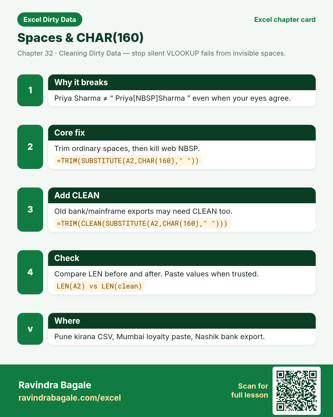
1. Extra spaces and non-breaking spaces (TRIM, CLEAN, SUBSTITUTE CHAR(160))
Friends, spaces are the number-one silent killer of VLOOKUP. Always TRIM, and remember CHAR(160) from web pages.
मित्रांनो, spaces मुळे VLOOKUP अनेकदा फसते. नेहमी TRIM करा, आणि वेबपेज मधल्या CHAR(160) चीही आठवण ठेवा.
दोस्तों, spaces की वजह से VLOOKUP अक्सर फेल होता है. हमेशा TRIM करें, और वेब पेज वाले CHAR(160) को भी याद रखें.
Why: Lookups and pivots fail when Priya Sharma and Priya Sharma look the same but are not.
What: Ordinary spaces, double spaces, and the invisible web space CHAR(160) that TRIM alone does not remove.
How:
- Select a helper column next to the dirty names.
- Type
=TRIM(A2)for normal spaces. - If VLOOKUP still fails, use
=TRIM(SUBSTITUTE(A2,CHAR(160)," ")). - Add
CLEANwhen imports from old systems bring control characters:=TRIM(CLEAN(SUBSTITUTE(A2,CHAR(160)," "))). - Copy the helper column → Paste Special → Values over the source when you trust it.
| Before | Formula / action | Result | Meaning |
|---|---|---|---|
Priya[NBSP]Sharma | =TRIM(SUBSTITUTE(A2,CHAR(160)," ")) | Priya Sharma | Retail order name from a Pune kirana CSV pasted from WhatsApp Web. |
2. Numbers stored as text
If SUM looks too small, suspect text-numbers before you blame the formula.
SUM खूप कमी दिसत असेल तर आधी text-numbers तपासा, formula ला दोष देऊ नका.
अगर SUM बहुत कम दिखे तो पहले text-numbers जाँचें, फॉर्मूला को दोष न दें.
Why: SUM ignores some text-numbers, and charts look empty even when you “see” digits.
What: Digits that Excel stores as text (green mark, left-aligned, or leading apostrophe).
How:
- Check with
=ISTEXT(B2)or look for the green corner. - Use
=VALUE(B2)or multiply by 1:=B2*1. - Or select the column → Data → Text to Columns → Finish (quick coerce).
- For many rows, add a helper, paste values, then delete the text column.
| Before | Formula / action | Result | Meaning |
|---|---|---|---|
'1250 | =VALUE(B2) | 1250 | Bank fee line from Nashik branch export saved as text. |
3. Text dates and mixed date formats
Never trust a date that still looks like text. Confirm with ISNUMBER, then lock the format.
जे तारीख अजून text वाटते तिच्यावर विश्वास ठेवू नका. ISNUMBER ने तपासा, नंतर format ठरवून टाका.
जो तारीख अभी भी text लगे उस पर भरोसा न करें. ISNUMBER से जाँचें, फिर format तय कर दें.
Why: India often sends DD/MM/YYYY while a US file sends MM/DD/YYYY. Excel may swap day and month quietly.
What: Dates stored as text, or real dates typed under the wrong regional format.
How:
- Ask: is this cell a real date or text? Try
=ISNUMBER(C2). - If text and your PC is DMY:
=DATEVALUE(C2)can work for15/03/2026. - Safer for mixed files: Data → Text to Columns → Date → pick DMY or MDY.
- Or split with LEFT/MID/RIGHT and rebuild with
=DATE(year,month,day). - Format the result as DD-MMM-YYYY so everyone reads the same day.
| Before | Formula / action | Result | Meaning |
|---|---|---|---|
3/15/2026 (US text) | Text to Columns → Date → MDY | 15-Mar-2026 | Manchester shop export opened on an Indian Windows locale. |
4. Inconsistent case and spelling
Fix categories before any Pivot. Clean words first, then count.
Pivot करण्याआधी categories स्वच्छ करा. आधी शब्द, मग count.
Pivot से पहले categories साफ़ करें. पहले शब्द, फिर count.
Why: PivotTables treat delivered, Delivered and DELIVERED as three statuses.
What: Mixed UPPER/lower and small spelling drift in categories.
How:
- Pick one style for categories (Title Case is fine for status).
- Use
=PROPER(TRIM(D2))or=UPPER(TRIM(D2)). - Build a small mapping table for spellings (e.g.
delivrd→Delivered) and look it up. - Replace values in Power Query when the list is long.
| Before | Formula / action | Result | Meaning |
|---|---|---|---|
delivered | =PROPER(TRIM(D2)) | Delivered | Logistics status from a Berlin lane CSV. |
5. Duplicate rows (Remove Duplicates, UNIQUE, COUNTIF flags)
Never delete duplicates blind. Flag, read two sample rows, then remove.
Duplicates थेट डिलीट करू नका. आधी flag करा, दोन rows वाचा, मग काढा.
Duplicates को सीधे डिलीट न करें. पहले flag करें, दो rows पढ़ें, फिर हटाएँ.
Why: Double invoices inflate sales. Healthcare and banking files often paste the same line twice.
What: Exact duplicate rows, or the same key repeated with tiny differences.
How:
- First create a flag:
=IF(COUNTIF($A$2:A2,A2)>1,"DUP","")on a key column. - Filter the flag and review before deleting.
- Data → Remove Duplicates on the key columns you choose.
- On Microsoft 365,
=UNIQUE(range)builds a clean spill list (LibreOffice: use Remove Duplicates or Advanced Filter). - Keep a backup sheet named
Before_Dedup.
| Before | Formula / action | Result | Meaning |
|---|---|---|---|
Priya Sharma row twice | COUNTIF flag then Remove Duplicates | One Priya row kept | Pune retail orders pasted twice from email. |
6. Blanks and missing values
A blank is data too. Write the rule in the About sheet.
रिकामे घर ही data आहे. नियम About sheet वर लिहा.
खाली सेल भी data है. नियम About शीट पर लिखें.
Why: Blank city or blank status breaks grouping and confuses averages.
What: Empty cells that mean “unknown”, “zero”, or “not applicable” — you must decide.
How:
- Count blanks:
=COUNTBLANK(E2:E100). - Decide a rule with the business: fill city from another column, type
Unknown, or leave blank on purpose. - For numeric blanks that should be zero in totals, use
=IF(F2="",0,F2)in a helper. - Do not fill medical or bank blanks with guesses without a written rule.
| Before | Formula / action | Result | Meaning |
|---|---|---|---|
City blank for Ravi | Flag or fill from branch master | Nashik or Unknown | Banking desk row missing city. |
7. Merged cells
Merged cells are for title banners, not for data tables.
Merged cells फक्त title साठी; data table मध्ये नको.
Merged cells सिर्फ टाइटल के लिए; डेटा टेबल में नहीं.
Why: Merged region labels look pretty but filters, sorts and pivots break.
What: Two or more cells joined into one visual block.
How:
- Select the merged block → Home → Merge & Center (click to Unmerge).
- Fill the empty cells downward (Home → Fill → Down) so every row has its Region.
- Never merge inside a data table you will Pivot.
- Use Center Across Selection for titles if you only need the look.
| Before | Formula / action | Result | Meaning |
|---|---|---|---|
West MH merged over two cities | Unmerge + Fill Down | West MH on each row | Kolhapur clinic patient summary. |
8. Combined columns to split (Text to Columns, Flash Fill, TEXTSPLIT)
Split before you SUM. Units never belong inside a number column.
SUM करण्याआधी split करा. Unit कधीही number column मध्ये नसावी.
SUM से पहले split करें. Unit कभी number कॉलम में न हो.
Why: Quantity and unit stuck together (5 kg) stop numeric totals.
What: One cell holding two facts that belong in two columns.
How:
- Easy menu: Data → Text to Columns → Delimited → Space.
- Flash Fill (Ctrl+E): type
5beside5 kg, fill down. - Formula fallback (works in LibreOffice too):
=VALUE(LEFT(A2,FIND(" ",A2)-1))and=TRIM(RIGHT(A2,LEN(A2)-FIND(" ",A2))). - Microsoft 365:
=TEXTSPLIT(A2," ")— keep the LEFT/FIND fallback for class PCs without it.
| Before | Formula / action | Result | Meaning |
|---|---|---|---|
5 kg | =VALUE(LEFT(A2,FIND(" ",A2)-1)) | 5 | Healthcare supply weight from Kolhapur clinic. |
9. Split columns to join
Prefer & when students have mixed Excel versions.
वेगवेगळ्या Excel versions साठी & सोप्पे आणि सुरक्षित.
मिश्र Excel versions के लिए & आसान और सुरक्षित है.
Why: First name and last name in two columns need one email label or one print line.
What: Joining text with &, CONCAT, or TEXTJOIN.
How:
- Simple and universal:
=A2&" "&B2. - Modern Excel:
=CONCAT(A2," ",B2). - Lists with commas: TEXTJOIN on Microsoft 365; on older Excel join with
&or use a helper. - TRIM the parts first so you do not create double spaces.
| Before | Formula / action | Result | Meaning |
|---|---|---|---|
Priya | Sharma | =A2&" "&B2 | Priya Sharma | IT ticket owner full name in Hyderabad desk. |
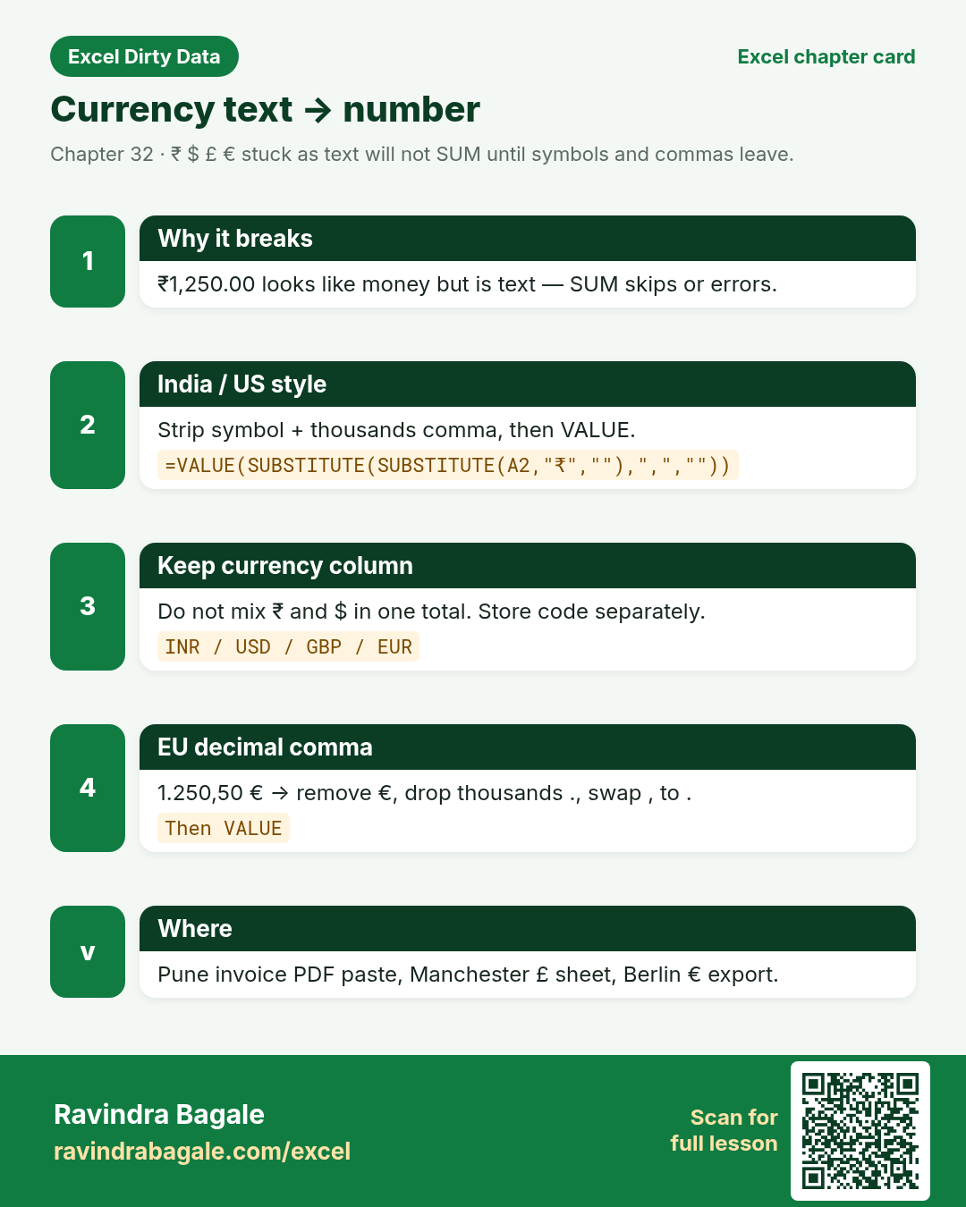
10. Currency symbols and thousand separators in text (₹ $ £ €)
Never SUM a column that still shows currency characters. Clean, then format as currency.
ज्या column मध्ये अजून currency चिन्ह आहे त्याचा SUM करू नका. आधी स्वच्छ, मग currency format.
जिस कॉलम में अभी भी currency चिह्न हो उसका SUM न करें. पहले साफ़ करें, फिर currency format.
Why: Text like ₹1,250.00 will not SUM until symbols and commas are removed.
What: Money pasted as text with symbols, commas, or European decimal commas.
How:
- Strip symbols with SUBSTITUTE (nest for many): remove ₹ $ £ € and spaces.
- Remove thousands commas:
=SUBSTITUTE(x,",","")for US/India style. - For
1.250,50 €(EU): remove €, replace.(thousands) with empty, replace,with., then VALUE. - Keep a separate Currency column (INR/USD/GBP/EUR) so you do not mix ₹ and $ in one sum.
- Example:
=VALUE(SUBSTITUTE(SUBSTITUTE(A2,"₹",""),",","")).
| Before | Formula / action | Result | Meaning |
|---|---|---|---|
₹1,250.00 | =VALUE(SUBSTITUTE(SUBSTITUTE(A2,"₹",""),",","")) | 1250 | Pune kirana invoice amount pasted from PDF. |
11. Units inside cells (“5 kg”)
Write the unit in the header, not inside every cell, once the column is clean.
Column स्वच्छ झाल्यावर unit header मध्ये लिहा, प्रत्येक सेल मध्ये नाही.
कॉलम साफ़ होने के बाद unit हेडर में लिखें, हर सेल में नहीं.
Why: Same as split — but people forget and multiply wrong (kg vs g).
What: Numbers glued to units.
How:
- Split qty and unit into two columns (see section 8).
- Convert units in a third column if needed: grams to kg = qty/1000.
- Validate with MAX/MIN — a “5000 kg” rice bag is probably grams mislabeled.
| Before | Formula / action | Result | Meaning |
|---|---|---|---|
5000 g | qty/1000 → kg | 5 kg | Logistics weight from Nagpur hub. |
12. Wrong data types
IDs and phone numbers are text, even when they look like digits.
ID आणि फोन नंबर text आहेत — दिसले तरी digits वाटले तरी.
ID और फोन नंबर text हैं — भले अंक दिखें.
Why: A phone number stored as a real number drops the leading zero. An ID becomes 4.5E+11.
What: Excel guessing Number vs Text vs Date incorrectly on import.
How:
- On import, set the column type in Text to Columns or Power Query to Text for IDs and phones.
- Prefix with apostrophe only as a quick fix:
'012345. - Use custom format if you must keep numeric storage but show leading zeros.
- Check TYPE/ISTEXT/ISNUMBER on a sample of 10 rows.
| Before | Formula / action | Result | Meaning |
|---|---|---|---|
StaffCode S01 vs 1 | Force Text on import | S01 kept | Banking staff codes from Dubai desk. |
13. Error values (IFERROR / IFNA)
IFERROR is a seatbelt, not a steering wheel. Fix the data too.
IFERROR सीटबेल्ट आहे, स्टीयरिंग नाही. Data पण दुरुस्त करा.
IFERROR सीटबेल्ट है, स्टीयरिंग नहीं. डेटा भी ठीक करें.
Why: #DIV/0! and #N/A scare managers and break dashboards.
What: Formula errors from zero hours, missing lookups, or bad VALUE() parses.
How:
- Fix the cause first (do not hide every error blindly).
- Wrap display formulas:
=IFERROR(D2/C2,"check hours"). - For lookups, prefer IFNA when you only want to catch #N/A.
- Keep a raw calc column and a clean display column if auditors need both.
| Before | Formula / action | Result | Meaning |
|---|---|---|---|
Cost/0 hours | =IFERROR(D2/C2,"check hours") | check hours | IT ticket cost rate in Hyderabad. |
15. Inconsistent codes
One master list for codes. Everything else is a defect.
Codes साठी एकच master list. बाकी सगळे defect.
Codes के लिए एक ही master list. बाकी सब defect.
Why: S01, s01 and S1 look like three staff members.
What: Codes with different case, padding, or obsolete values (S99).
How:
- UPPER or PROPER the code column.
- Pad with TEXT or RIGHT:
="S"&RIGHT("00"&number,2)when needed. - Match against a staff master with exact match only.
- Flag unknowns:
=IF(COUNTIF(Master[Code],A2)=0,"bad code","").
| Before | Formula / action | Result | Meaning |
|---|---|---|---|
s01 | =UPPER(A2) | S01 | Nashik banking timesheet codes. |
16. Outliers
Outliers are questions, not automatic deletes.
Outlier म्हणजे प्रश्न; त्वरित delete नाही.
Outlier मतलब सवाल; तुरंत delete नहीं.
Why: One row with 1,000,000 ₹ or 40 hours can break averages and charts.
What: Values far from the normal range — sometimes real, sometimes typos.
How:
- Sort the column or use MIN/MAX.
- Compute a simple fence: flag if value > 3× median (classroom rule of thumb).
- Talk to the owner before deleting — Priya’s 1,000,000 may be a real annual invoice.
- Keep an OutlierFlag column instead of silent deletes.
| Before | Formula / action | Result | Meaning |
|---|---|---|---|
Cost_INR 1000000 | OutlierFlag = Cost high | Review with manager | IT ticket cost typo vs real project fee. |
17. Header rows in the middle
One header at the top. Everything else is a data row — or junk.
वर एकच header. बाकी data row — किंवा junk.
ऊपर एक ही header. बाकी data row — या junk.
Why: A repeated header or a “Total” row in the middle breaks sorts and pivots.
What: Batch titles pasted again inside the data.
How:
- Filter the first column for the word
BatchorTotaland delete those rows. - In Power Query: filter rows where SKU column does not equal
SKU. - Reload a clean extract from the source system when possible.
| Before | Formula / action | Result | Meaning |
|---|---|---|---|
Row repeating Batch/SKU/City… | Filter out header-like rows | Only real SKUs left | Retail stock paste from Pune + Manchester. |
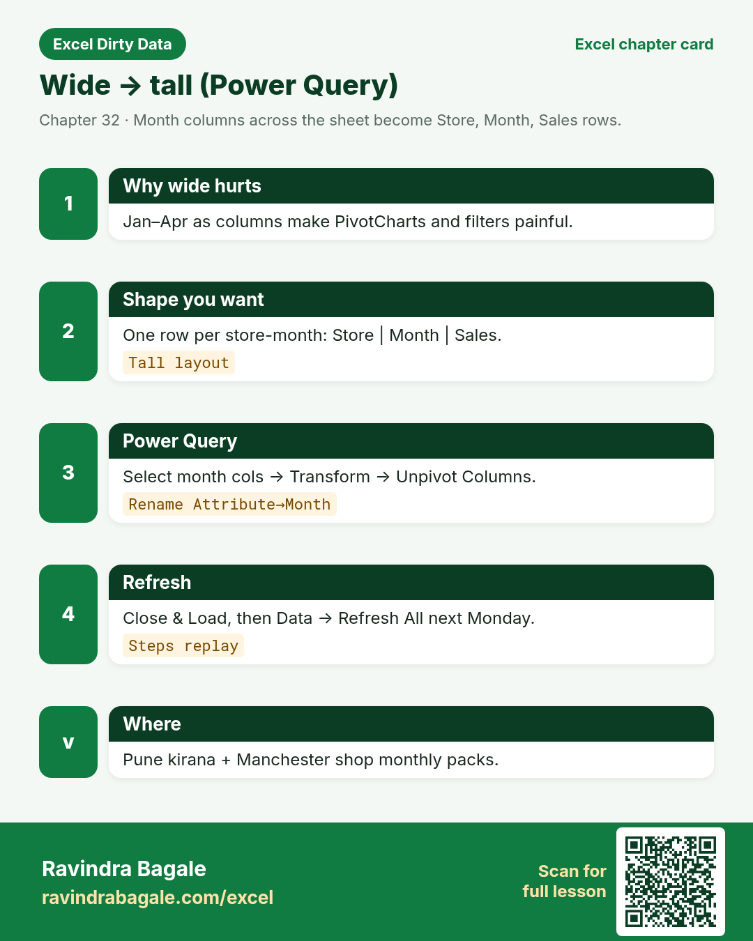
18. Wide vs tall data (unpivot)
Wide is for reading by humans; tall is for PivotTables.
Wide माणसांना वाचायला; tall PivotTables साठी.
Wide इंसानों को पढ़ने के लिए; tall PivotTables के लिए.
Why: Months across columns (Jan–Apr) make PivotCharts painful.
What: Wide layout vs tall layout (Store, Month, Sales).
How:
- Prefer tall data for analysis: one row per store-month.
- In Power Query: select month columns → Transform → Unpivot Columns.
- Rename Attribute → Month, Value → Sales.
- Close & Load to a new sheet.
| Before | Formula / action | Result | Meaning |
|---|---|---|---|
Store | Jan | Feb | Mar | Unpivot month columns | Store | Month | Sales | Pune kirana + Manchester shop monthly sales. |
19. Power Query cleaning checklist
If you clean the same file every Monday, stop pasting formulas — build a query.
दर सोमवारी तेच clean करत असाल तर query बनवा; दरवेळी formula पेस्ट करू नका.
अगर हर सोमवार वही सफ़ाई करते हैं तो query बनाएँ; हर बार formula पेस्ट न करें.
Why: Repeating the same TRIM/VALUE fixes every week wastes time. Power Query remembers the steps.
What: A refreshable cleaning pipeline: Get Data → transform → Close & Load.
How:
- Data → Get Data → From File / From Folder (or From Clipboard for class demos).
- Remove top junk rows; promote headers.
- Transform → Format → Trim / Clean on text columns.
- Replace values for status spellings; set data types (Date, Decimal, Text).
- Remove duplicates on business keys; unpivot wide months if needed.
- Home → Close & Load To… Table on a new sheet.
- Next week: Data → Refresh All — steps replay automatically.
| Before | Formula / action | Result | Meaning |
|---|---|---|---|
Weekly dirty CSV | Power Query steps saved | Clean table on Refresh | Banking + retail weekly ops pack. |
Practice tasks (12)
Use dirty-data-practice.xlsx. Check ideas against dirty-data-solution.xlsx. Avoid XLOOKUP / TEXTJOIN / TEXTSPLIT in checks so LibreOffice class PCs keep up — fallbacks are in the lesson.
- On Raw_Import, create Name_Clean with TRIM + SUBSTITUTE CHAR(160) for customer names.
Hint
Start with Priya in row 2 — LEN should drop.
- Convert Amount_Text for Priya into a real number 1250.
Hint
Strip ₹ and commas, then VALUE.
- Parse Qty_Unit “5 kg” into Qty=5 and Unit=kg with LEFT/FIND (no TEXTSPLIT).
Hint
FIND the space.
- Normalise Status to Title Case with TRIM.
Hint
PROPER(TRIM(...)).
- Flag duplicate Priya rows with COUNTIF.
Hint
Same name + date + amount is a clue.
- Fix the US date 3/15/2026 so it becomes 15-Mar-2026 on an Indian PC.
Hint
Text to Columns → MDY.
- Unmerge Region on Merged_Trap and fill West MH down.
Hint
Unmerge, then Fill Down.
- Remove the middle header row and the Total row on Mid_Headers.
Hint
Filter text “Batch” / “Total” in column A carefully.
- Unpivot Wide_Months into Store, Month, Sales (Power Query or manual copy).
Hint
Four month columns become rows.
- Wrap the #DIV/0! on Errors_Outliers with IFERROR.
Hint
Show “check hours” when hours are 0.
- Flag StaffCode S99 as invalid using a small master list S01–S05.
Hint
COUNTIF against the master.
- Write one business rule on About this data for blank cities.
Hint
Unknown vs fill-from-branch — pick one and document it.
Quick quiz
Q1. TRIM alone always removes the web non-breaking space CHAR(160).
Q2. Best first check that a date cell is a real date?
Q3. ₹1,250.00 as text — what is a LibreOffice-safe cleanup path?
Q4. Why are merged cells bad inside a data table?
Q5. Wide month columns should usually become…
Q6. IFERROR should be used to…
Q7. Duplicate cleanup — safest classroom habit?
Q8. “5 kg” in one cell — good analysis shape is…
Loading practice tasks...
- Total amount (Easy): Add up Amount in D2:D11.
- Average qty (Easy): Average of the Qty column, rounded to 2 decimals.
- Delivered rows (Easy): How many rows have Status "Delivered"?
- Blank check (Easy): Count blank cells in C2:C11.
- Delivered amount (Medium): Total of D where C is "Delivered".
- Pune delivered qty (Medium): Total of E where B is "Pune" and C is "Delivered".
- Largest pending (Medium): Largest D where C is "Pending".
- Row 2 value (Medium): Multiply the first-row Amount (₹) by the first-row Qty.
- Look up Ananya Iyer (Medium): The Amount for "Ananya Iyer".
- Total value (Hard): Sum of D times E for all rows.
- Share delivered (Hard): Share of D that is Delivered, rounded to 3 decimals.
- Trim test name (Hard): Trim " Priya Sharma " (spaces outside).
Quick revision cards (sample of 3)
Approved Excel card style: standalone, no tip/photo section, QR to this lesson. Full card set can expand at deploy.
Marathi / Hindi plan
English chapter is live. Marathi twin planned at /mr/excel/ch32-cleaning-dirty-data-in-excel/ with the same structure, absolute /excel/... and /mr/excel/... links, and keep teacher tabs EN/MR/HI on both. Hindi remains available in the teacher tabs on the English URL (site pattern).