Chapter 33
Conditional Formatting: Complete Guide
Learn every major Conditional Formatting tool in Excel — highlight rules, text and blanks, colour scales, data bars, icon sets, and formula rules that paint whole rows. Practice file includes working rules you can edit.
Ravindra Bagale’s Tip
Open the practice workbook first. Change a number and watch the colour move — that is how CF teaches itself.
Ravindra Bagale’s Tip – मराठी
आधी प्रॅक्टिस वर्कबुक उघडा. अंक बदला आणि रंग कसा बदलतो ते पाहा.
Ravindra Bagale’s Tip – हिंदी
पहले प्रैक्टिस वर्कबुक खोलें। संख्या बदलें और रंग कैसे बदलता है देखें।
https://ravindrabagale-cards.s3.ap-south-1.amazonaws.com/excel/ch33/ch33-cf-practice.xlsx.1. Why conditional formatting matters
CF is a spotlight. You still need good data — CF only shows what is already there.
कंडीशनल फॉरमॅटिंग म्हणजे स्पॉटलाइट. डेटा चांगला असेल तरच रंग अर्थपूर्ण दिसतात.
कंडीशनल फ़ॉर्मैटिंग स्पॉटलाइट है। डेटा सही हो तभी रंग का मतलब समझ में आता है।
Why: Numbers alone are easy to skim past. Colour and icons make risks and wins jump out in a meeting.
What: Conditional Formatting (CF) paints cells when a rule is true — greater than, text contains, formula, colour scale, data bar, or icon set.
How:
- Open a sheet with numbers or status text (sales, scores, stock days).
- Ask: what should a manager notice in three seconds?
- Apply one clear CF rule per question — avoid rainbow overload.
- Test by changing a value and watching the colour update.
| Before / setup | Rule or formula | Result | Meaning |
|---|---|---|---|
Orders 55 vs 9 | Highlight Cells > Greater Than 50 | 55 green, 9 unchanged | High-volume reps stand out |
2. Highlight Cells Rules (number, text, date, duplicate)
Start with Highlight Cells Rules. They cover 80% of daily work.
रोजच्या कामात Highlight Cells Rules पुरेसे असतात — इथून सुरुवात करा.
रोज़ के काम में Highlight Cells Rules काफी हैं — यहीं से शुरू करें।
Why: You need red/amber/green flags without writing formulas.
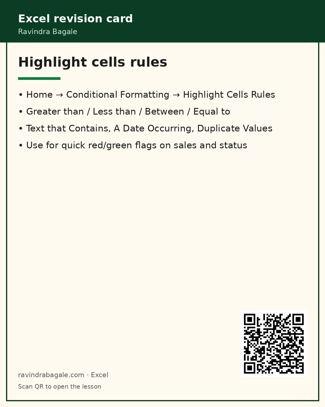
What: Home → Conditional Formatting → Highlight Cells Rules: Greater Than, Less Than, Between, Equal To, Text that Contains, A Date Occurring, Duplicate Values.
How:
- Select the values (example: Revenue column D2:D9).
- Home → Conditional Formatting → Highlight Cells Rules → Less Than…
- Type 20000, pick Light Red Fill, OK.
- Repeat for Status Equal To “Risk” with yellow fill.
- For duplicates: select Ticket IDs → Duplicate Values.
| Before / setup | Rule or formula | Result | Meaning |
|---|---|---|---|
Revenue INR 15000 | Less Than 20000 → red fill | Cell turns red | Low revenue risk flag |
3. Text contains and blank cells
Blank rules catch incomplete forms before you mail the file.
रिकाम्या सेलचे नियम अपूर्ण फॉर्म पकडतात.
खाली सेल वाले नियम अधूरे फ़ॉर्म पकड़ते हैं।
Why: Notes and owner columns hide missing data and urgent words.
What: Use Text that Contains for keywords, or a formula rule =B2="" for blanks.
How:
- Select the Note column.
- Highlight Cells Rules → Text that Contains… → type urgent.
- For blanks: Conditional Formatting → New Rule → Use a formula → =B2="" (adjust column).
- Choose a fill so empty owners cannot be ignored.
| Before / setup | Rule or formula | Result | Meaning |
|---|---|---|---|
Note: Contains urgent word | Text contains “urgent” | Orange fill | Keyword catcher |
4. Colour scales (heat maps)
Colour scales are perfect for inventory days and exam averages.
इन्व्हेंटरी दिवस आणि गुणांसाठी कलर स्केल उत्तम.
इन्वेंटरी दिनों और अंकों के लिए कलर स्केल बहुत ठीक है।
Why: You want a gradient from worst to best without many separate rules.
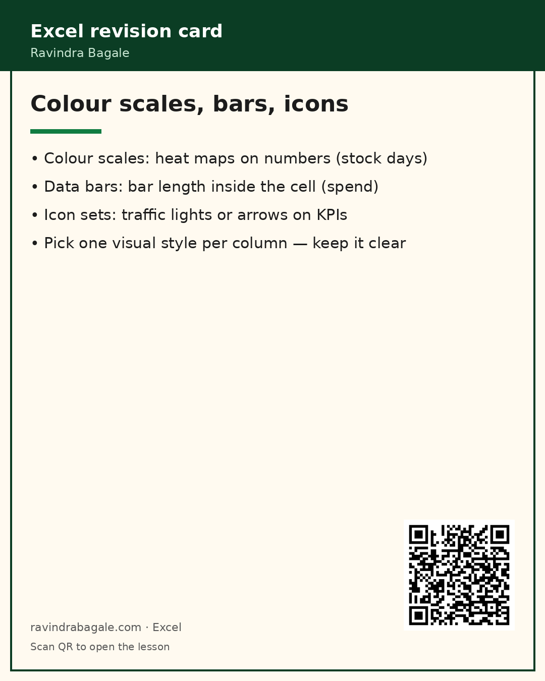
What: Colour Scales shade from a low colour through mid to high (often red → yellow → green).
How:
- Select the number range (Days of cover).
- Conditional Formatting → Color Scales → pick a 3-colour scale.
- Manage Rules → Edit Rule to set min / mid / max numbers if needed.
- Use one scale per sheet area so colours mean the same thing.
| Before / setup | Rule or formula | Result | Meaning |
|---|---|---|---|
Days of cover 2 … 45 | 3-colour scale red–yellow–green | Low days red, high green | Stock heat map |
5. Data bars
Data bars beat a separate chart when space is tight.
जागा कमी असेल तर डेटा बार चार्टपेक्षा सोयीचे.
जगह कम हो तो डेटा बार चार्ट से आसान हैं।
Why: You want bar-chart length inside the cell for quick compare.
What: Data Bars draw a bar proportional to the value in the same cell.
How:
- Select Spend USD values.
- Conditional Formatting → Data Bars → Solid Fill (or Gradient).
- Edit Rule to show bar only, or bar + value.
- Keep the column number format (currency) readable.
| Before / setup | Rule or formula | Result | Meaning |
|---|---|---|---|
Spend 1500 … 9100 USD | Data bar blue | Longer bar = higher spend | Inline mini chart |
6. Icon sets (traffic lights, arrows)
Match thresholds to your real targets — do not leave the default if your pass mark differs.
थ्रेशहोल्ड तुमच्या खऱ्या लक्ष्यांनुसार सेट करा.
थ्रेशहोल्ड अपने असली लक्ष्य के हिसाब से सेट करें।
Why: KPIs need symbols managers already understand.
What: Icon Sets place traffic lights, arrows, or ratings beside (or instead of) the number.
How:
- Select Score % cells.
- Conditional Formatting → Icon Sets → 3 Traffic Lights.
- Manage Rules → Edit → set thresholds (example: ≥67 green, ≥33 yellow, else red).
- Tick “Show Icon Only” if the number is shown elsewhere.
| Before / setup | Rule or formula | Result | Meaning |
|---|---|---|---|
Score 92%, 61%, 45% | 3 Traffic Lights by percent | Green / yellow / red icons | KPI status at a glance |
7. Formula rules and whole-row highlight
The $ before the column letter keeps the test on one column while you paint many columns.
$ स्तंभ अक्षरासमोर ठेवा — एक स्तंभ तपासा, अनेक रंगवा.
$ कॉलम अक्षर से पहले रखें — एक कॉलम जाँचें, कई रंगें।
Why: Built-in rules cannot highlight an entire row when one column fails.
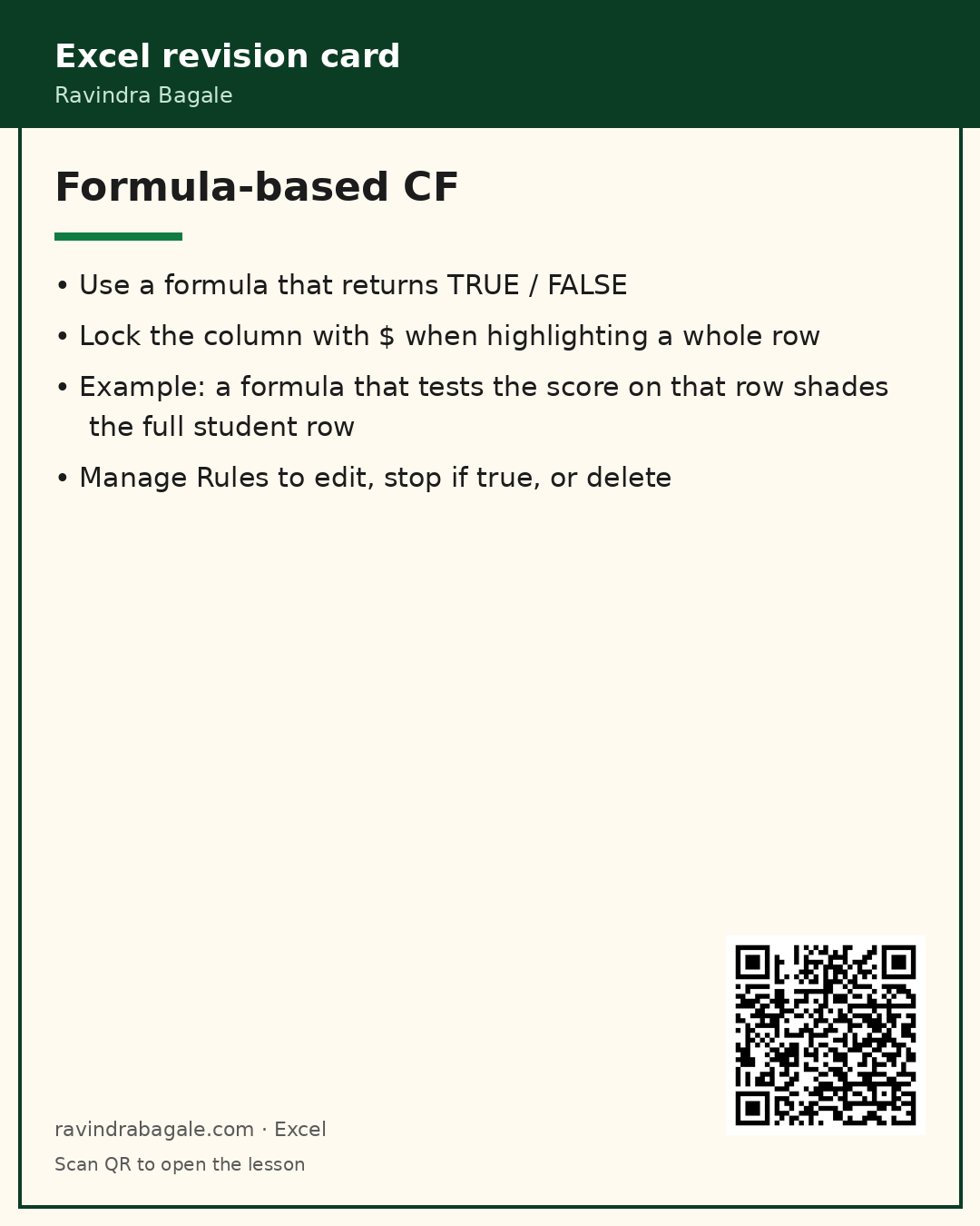
What: New Rule → Use a formula to determine which cells to format. Return TRUE to format.
How:
- Select the full table body A2:E7 (not only one column).
- New Rule → Use a formula → enter =$E2<60 (lock column E with $).
- Set a light red fill → OK.
- Add a second rule =$E2=MAX($E$2:$E$7) with green for the top average.
- Open Manage Rules → stop if true if rules should not stack.
| Before / setup | Rule or formula | Result | Meaning |
|---|---|---|---|
Average column E | =$E2<60 on A2:E7 | Whole row red when fail | Row-level attention |
8. Manage, edit, clear, and copy CF
If colours look wrong, open Manage Rules before you add yet another rule.
रंग चुकीचे वाटत असतील तर नवा नियम जोडण्यापूर्वी Manage Rules उघडा.
रंग गलत लगें तो नया नियम जोड़ने से पहले Manage Rules खोलें।
Why: Rules pile up and fight each other.
What: Manage Rules lists every rule on the sheet. You can edit, delete, reorder, and stop if true. Paste Special → Formats copies CF.
How:
- Home → Conditional Formatting → Manage Rules… (set “This Worksheet”).
- Edit a rule or Delete as needed. Drag order — top rules run first.
- To clear: Clear Rules → From Selected Cells or Entire Sheet.
- To copy: Copy cell → Paste Special → Formats (includes CF).
| Before / setup | Rule or formula | Result | Meaning |
|---|---|---|---|
Too many rules | Manage Rules → delete / reorder | Clean rule list | Stable colours |
Practice tasks (12)
- On HighlightCells, change Omar Farouk Orders from 61 to 40. Which CF colours change?
Hint
Watch the Orders column green/blue rules.
- Add a Greater Than rule on Revenue for values over 300000 with green fill.
Hint
Highlight Cells Rules → Greater Than.
- On TextAndBlank, type urgent into Neha’s blank note — confirm the text rule fires.
Hint
Text contains rule is on column D.
- Create a Duplicate Values rule on City in HighlightCells (copy the sheet first if you like).
Hint
Highlight Cells → Duplicate Values.
- On ColorScale, edit the rule so mid point is fixed at 15 days.
Hint
Manage Rules → Edit → Number midpoint.
- On DataBars, switch to Show Bar Only and note how the number hides.
Hint
Edit Rule → Show Bar Only.
- On IconSets, reverse the icon order and explain when reverse helps.
Hint
Edit Rule → Reverse Icon Order.
- On FormulaRules, change Devika’s Math to 90 — does her row leave the red rule?
Hint
Average must rise to 60+.
- Add a formula rule that greens any row where Science ≥ 90.
Hint
=$D2>=90 on A2:E7.
- On YourTasks, apply a colour scale to Qty and a Greater Than 5000 rule on Line total.
Hint
Select ranges then add two separate rules.
- Copy CF from HighlightCells Status column to a new column Flag using Paste Special Formats.
Hint
Copy → Paste Special → Formats.
- Clear all rules from YourTasks after you finish practising.
Hint
Clear Rules → Entire Sheet on that sheet.
Quick quiz
Q1. Where do you find Conditional Formatting?
Q2. Which rule type paints a heat map across many numbers?
Q3. To highlight a whole row when Average in E is under 60, which formula is best?
Q4. Duplicate Values is under which menu?
Q5. Data bars show…
Q6. “Stop If True” is set in…
Q7. Text that Contains “urgent” needs…
Q8. Paste Special → Formats will…
End-of-chapter checklist
- I can apply Greater Than / Less Than / Between / Equal To / Text Contains / Duplicate rules.
- I can build a colour scale, data bars, and an icon set with sensible thresholds.
- I can write a formula rule with
$to shade a whole row. - I can Manage, Clear, and Paste-Special copy CF.
Quick revision cards (sample of 3)
Approved Excel card style: standalone, QR to this lesson. Full set can expand at deploy. Cards hosted on S3.